
This blog is adapted from
Traveling Waves Integrate Spatial Information Through Time
Traveling Waves Integrate Spatial Information Through Time
March 10, 2025The act of vision is a coordinated activity involving millions of neurons in the visual cortex, which communicate over distances spanning up to centimeters on the cortical surface. How do these neurons perform this coordinated computation and effectively share information over such long distances?
Traveling Waves in the Brain
Traveling waves of neural activity have been observed throughout the brain, spanning a range of scales and brain regions (Muller et al., 2018)[1]. Surprisingly, these waves have even been measured in visual cortex in response to stimuli, propagating over the otherwise highly spatially organized visual field (Cowey, 1964)[2]. Recent advances in recording technologies, such as calcium imaging and multielectrode arrays, have allowed neuroscientists to measure these waves with unprecedented precision (Muller et al., 2014)[3], (Davis et al., 2020)[4]; however, due to the inherent complexity of these measurements and the multitude of potential confounding variables, elucidating a causal role for these dynamics has remained highly challenging – especially in the context of vision.
A leading hypothesis suggests these waves may transfer and combine information across spatially distant regions of the visual cortex (Sato et al., 2012)[5]. For example, Kitano et al. (1994)[6] and Bringuier et al. (1999)[7] found that neurons could be elicited to respond to stimuli far outside their classical receptive fields, but with an increased delay as a function of distance – as if the information was slowly transmitted over time between adjacent neurons. Despite these promising observations, it still remains unclear how neurons might actually use this long-range information, leading many to argue that these effects are largely ’epiphenomenal’; in other words, they are resulting from some separate causal process without any causal role of their own.
In a recent preprint (Jacobs et al. 2025)[8], we take a machine learning approach to directly measure the computational role of traveling waves in the spatial integration of information. Specifically, we introduce a set of convolutional recurrent neural networks that can generate traveling waves in their hidden states when processing visual inputs. We observe that these waves effectively expand neurons’ receptive fields, allowing distant features within an image to be shared more readily between neurons with otherwise locally constrained receptive fields. We demonstrate that these models tackle visual segmentation tasks requiring global integration, outperforming local feed-forward models and even rivaling the popular non-local U-Net architecture (Ronneberger et al., 2015)[9] (now used in virtually all diffusion models) — despite having fewer parameters. In the following blog post, we will give a high-level overview of this work and the motivational theory.
What does it mean to “Integrate Spatial Information”?
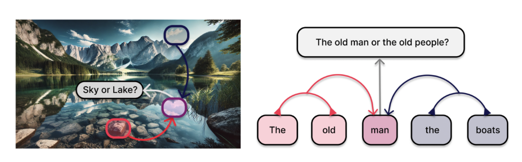
At the simplest level, the integration of spatial information means that a neuron at one spatial location has access to signals from far-flung regions of the input. For an image, that could mean that a neuron at the bottom of an image is able to use information from the top of the image in order to figure out if the given blue patch it is looking at is part of the sky, or just a reflection off a lake; while for language, it might involve linking words from the beginning and end of a sentence to figure out the meaning of a word in the middle (Figure 2).
Modern artificial vision systems do not use anything like wave dynamics to integrate spatial information. Instead, most systems use a large number of layers (such as deep convolutional neural networks), bottleneck layers (such as in U-Nets), and global connectivity (such as in the all-to-all attention of Transformers). However, each of these approaches comes with its own limitations. For example, deeper networks have more challenging gradient propagation (requiring the use of residual connections), bottlenecks inherently limit the capacity of neural representations (requiring U-Net like skip connections), and all-to-all global connectivity is extremely computationally expensive (in terms of run time and memory usage, limiting scalability).
In this work, we seek to answer if traveling wave integration of spatial information might be an efficient biologically plausible alternative to these methods. Furthermore, practically, how might waves actually be doing this integration? Specifically, in what format is this information transmitted such that downstream neurons can best read it out?
How Might Waves Integrate Spatial Information?
One well known mechanism by which waves can be seen to integrate spatial information is exemplified by the famous mathematical question, posed by Mark Kac in (1966): ”Can One Hear the Shape of a Drum?”[10]. At a high level, Kac wondered whether the set of natural frequencies at which a drum head vibrates is uniquely determined by the shape of its boundary.
Intuitively, when you strike a drumhead, the initial disturbance will propagate outwards as a transient traveling wave until it reaches the fixed boundary conditions where it will reflect with a phase shift. This reflected wave will thus have collected information about the boundary, and serves to bring it back towards the center. After repeated reflections and collisions, the wave activity eventually settles into patterns (normal modes) determined by the drumhead’s global geometry.
In a broad sense then, the answer to the famous questions is yes, the shape of a drum does determine the sound that it will produce (but not always uniquely, see (Gordon et al., 1992)[11] for the famous counter example of ‘isospectral drum shapes’).
In the videos below we show a simulation of these dynamics precisely for square drum heads of different sizes.
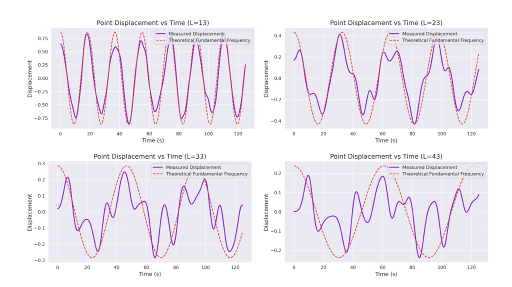
But how exactly is the drum’s geometry encoded in these wave dynamics? Taking inspiration from Kac’s famous question, in Figure 3 we look at the ‘sound’ of these waveforms through the time-series of the drumhead’s displacement at a chosen point on the drum, for example from a point just off the center.
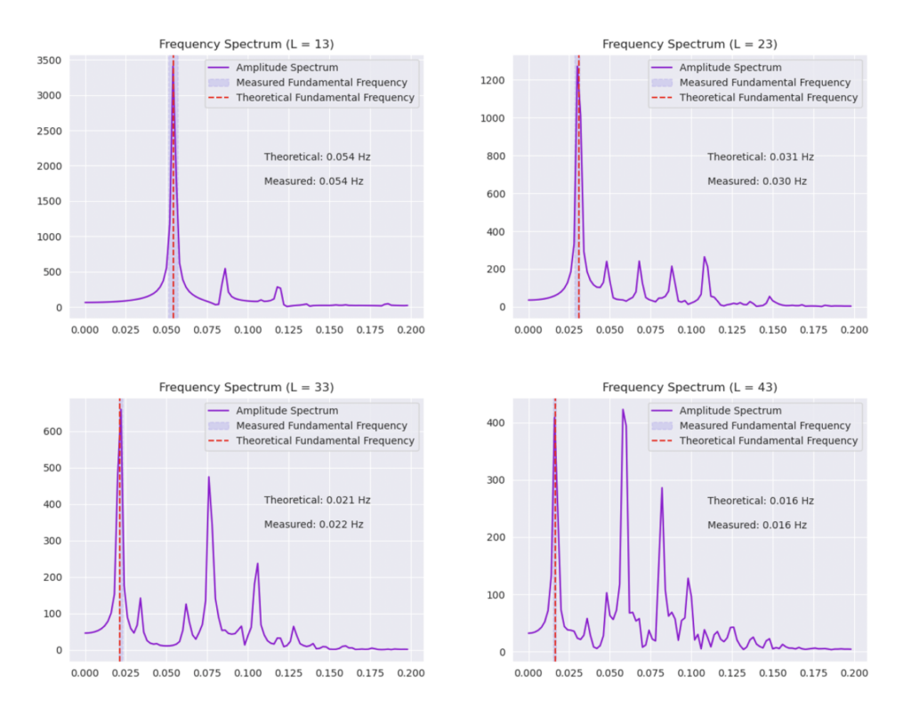
Often, a more natural way to think about sound is in terms of its frequency components, which we can compute by taking the Fourier transform of the displacement. In doing so, we arrive at the ‘spectral representations’ of each shape, which we plot in Figure 4. Mathematically, for a square drum, one can derive that the lowest frequency at which a drum head will vibrate is inversely proportional to its side length – and indeed, if we look at the first peak in the frequency spectra plotted, we can see that they gradually shift lower as the side lengths increase. This aligns with our real-world intuition that larger drums make deeper, lower-pitched sounds.
But how could these ideas possibly relate to the brain or even artificial neural networks? First, we note that the equation which we used to simulate the above dynamics (the wave equation[12]) actually appears very similar to the equations describing the time evolution of a recurrent neural network hidden state when discretized over space and time (as noted by other authors such as (Keller et al. 2024)[13] and (Hughes et al. 2019)[14]). Secondly, from this conceptual framework, we can see the desired ’integrated information’ is actually only present in the time-series history of activity at each location, and best read out through a linear transformation of this history (e.g. through the Fourier Transform).
Taking inspiration from this analogy, in our recent work, we therefore propose to investigate whether wave-based RNN architectures might similarly be able to integrate spatial information into temporally extended representations.
Can a Wave-based RNN Hear the Shape of a Polygon?
To begin, we start with the simplest learned variant of this question: Can A Wave-based RNN Hear the Shape of a Polygon?
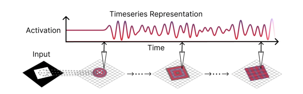
To test this we provide images of black polygons on white backgrounds to a wave-generating RNN architecture, and measure the Fourier coefficients of the resulting dynamics at each point. We then train the model to use this ‘spectral representation’ at each pixel location to classify the pixel as either belonging to the background or one of the n-sided shapes. For each of the shapes, the model must crucially know which shape it is a part of (e.g. triangle vs. square vs. hexagon), a task which requires a significantly larger portion of the image to be able to accomplish successfully, compared with each neuron’s immediate single-step receptive field (analogous to the examples in Figure 2 above).
In Figure 5, we show the resulting wave-dynamics learned by the model on an example hexagon image. We see the model has learned to use differing natural frequencies inside and outside the shape to induce soft boundaries, causing reflection, thereby yielding different internal dynamics based on shape.
In Figure 6 (below), we show the resulting predicted segmentation masks, and a select set of Fourier coefficient magnitudes at all spatial locations for an example image of a triangle and a hexagon. We see that the model does indeed learn to accomplish this segmentation task, and further separates different shapes into different parts of frequency space. On the right, we plot the full frequency spectrum for each shape in the dataset, averaged over all pixels containing that class label. We see that different shapes have qualitatively different frequency spectra, allowing for > 99% pixel-wise classification accuracy on a test set.
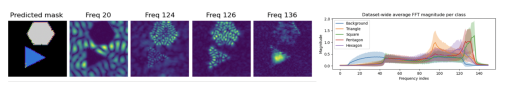
Plot of predicted semantic segmentation and select set of frequency bins for each pixel of a
given test image. (Right) The full frequency spectrum for each shape in the dataset.
In a sense then, this model can actually be understood to be ‘hearing the shape’ of each polygon, by propagating waves around it in latent space, and extracting the Fourier coefficients of the resulting oscillations. To see what we mean, take a listen for yourself. Below are the different sounds that the model has learned to produce foreach of the shapes in the dataset, synthesized from the above Fourier spectra, as well as for the background:

Background

Hexagon

Pentagon

Square

Triangle
Scaling It Up: Semantic Segmentation
Finally, we tested whether this principle remains effective on more complex segmentation tasks. To do this, we use datasets such as Tetrominoes, and variants of MNIST to see how well our models might be able to segment the images. Again, crucially, for our models of interest we limit the immediate feed-forward and recurrent receptive fields of each neuron to a small local neighborhood, meaning that if the model learns to correctly segment each pixel as belonging to its correct larger shape, it must be integrating global information through recurrent dynamics.
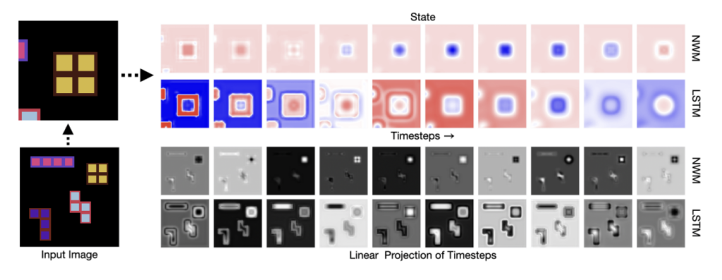
In Figure 7 below, we demonstrate these results for Tetrominoes and two of the locally-constrained RNNs we tested – one with a bias towards wave dynamics (the Neural Wave Machine (Keller et al. 2024)[15]), and another standard recurrent neural network with no such bias (a convolutional LSTM). Incredibly, despite having no initial inductive bias towards generating waves, we see the LSTM model learns to generate waves to solve this task – implying a degree of optimality to a wave-based solution. Below, we show videos of the LSTM wave dynamics:
Comparing Timeseries Representation Readouts
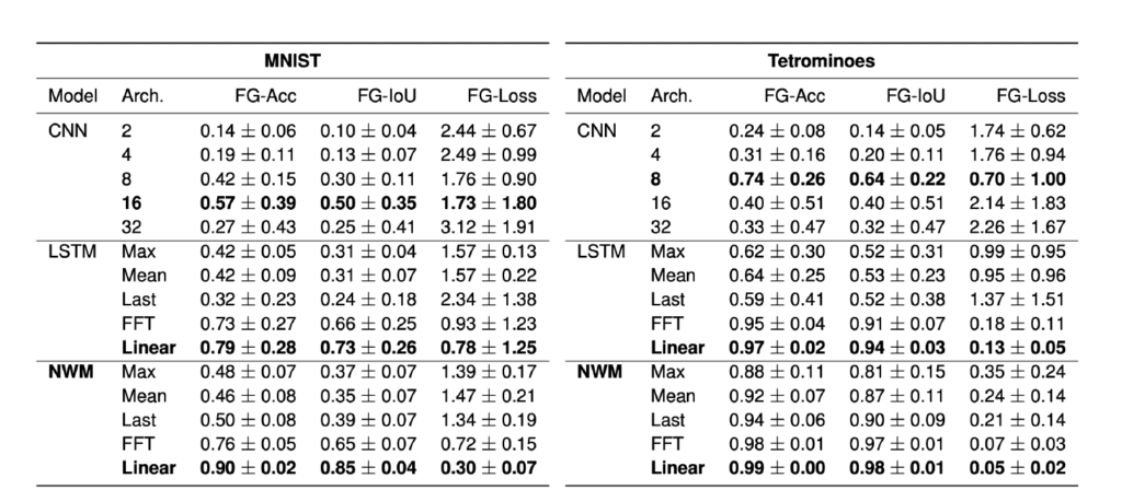
To answer the question of how global information might best be represented by traveling waves, we also compare different types of linear transformations of the hidden state time series to see which is the best for reading out the semantic labels. In Table 8, we see that, in line with our expectations, more complex linear transformations of the hidden state timeseries are the most powerful for extracting the global information, with an arbitrary learned linear transformation outperforming the Fourier transform (FFT) and mean or max pooling over time. We see that these linear transformations over time also dramatically outperform simply taking the ’last’ hidden state of the RNN, a common technique when using RNNs to integrate information, thereby suggesting we take a second look at traditional RNN literature and methods for integrating spatial information.
Comparing Wave-based Integration with CNN Depth
To answer how this wave-based integration of information compares with more common alternatives, in Table 8 we additionally compare with convolutional neural networks of varying depths on the same task. Critically, we see that CNNs with small receptive fields (small numbers of layers) are unable to segment these images as expected, while deeper models are sometimes able to solve the task, but are generally more unstable yielding lower average performance and significantly higher variance over 10 random seeds. While preliminary, these results imply that wave-based integration of information may be a stable and robust alternative to network depth in locally constrained systems.
Comparing Wave-based Integration with U-Nets
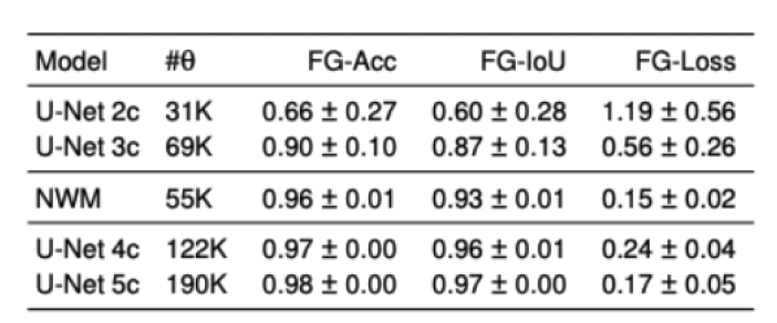
Finally, we test on a variant of MNIST with multiple digits per image, hypothesizing that the increased information required to simultaneously represent all digits may be challenging for U-Net architectures with limited numbers of channels (while this wouldn’t be the case for wave-based models which operate over all pixels in parallel). In Table 9 we show the results of this final experiment, where we see that indeed, the wave-based models appear to outperform U-nets of comparable size, despite having fewer parameters. We hypothesize that this is likely due to wave-based models leveraging the parallel processing ability of wave dynamics, and the lack of a spatial bottleneck in their integration of information. Videos of these wave dynamics are shown below:
Conclusion
In summary, our findings suggest that traveling wave-based neural architectures offer a compelling and biologically plausible alternative to traditional methods such as deep convolutional networks, bottleneck layers, or all-to-all self-attention for spatial information integration. By producing traveling waves, these models expand local receptive fields and encode global information efficiently through their timeseries representations.
Our traveling wave-based approach not only enables effective segmentation in challenging visual tasks with fewer parameters, but also aligns more closely with the distributed processing observed in the brain. These unique frequency-space representations provide a promising avenue for drawing parallels between artificial models and neural recordings from modalities like MEG and EEG.
As we move forward, exploring these models further could unlock new avenues for understanding brain function and designing efficient, scalable machine learning systems that leverage the inherent advantages of wave dynamics.
Note: An earlier version of this manuscript was accepted to the ICLR Re-Align workshop.
- https://www.nature.com/articles/nrn.2018.20[↩]
- https://journals.physiology.org/doi/abs/10.1152/jn.1964.27.3.366[↩]
- https://www.nature.com/articles/ncomms4675[↩]
- https://www.nature.com/articles/s41586-020-2802-y[↩]
- https://www.cell.com/neuron/fulltext/S0896-6273(12)00591-0[↩]
- https://pubmed.ncbi.nlm.nih.gov/7947408/[↩]
- https://www.science.org/doi/abs/10.1126/science.283.5402.695[↩]
- https://arxiv.org/abs/2502.06034[↩]
- https://arxiv.org/abs/1505.04597[↩]
- https://www.jstor.org/stable/2313748[↩]
- https://arxiv.org/abs/math/9207215[↩]
- https://en.wikipedia.org/wiki/Wave_equation[↩]
- https://openreview.net/forum?id=p4S5Z6Sah4[↩]
- https://www.science.org/doi/10.1126/sciadv.aay6946[↩]
- https://proceedings.mlr.press/v202/keller23a.html 6[↩]