A Dynamical Model of Neural Scaling Laws

Over the past several years, advances in deep learning have shown that large models continue to improve as training time, dataset size and model size increase ^{[1][2][3][4][5][6]}. Understanding the rate of improvement of these systems with an increase in these resources is crucial if one desired to scale up model size and training time in a compute optimal manner.³ Empirically, several studies have found the loss for a network with 𝑡 update steps and 𝑁 parameters can be decently approximated as a power law^2-6 in each of these quantities.

$$\mathcal L = C_t \ t^{-\alpha_t} + C_N N^{-\alpha_N} + \mathcal L_{\infty}.$$

The constants $C_t, C_N$ and exponents $\alpha_t$ and $\alpha_N$ and asymptote $\mathcal L_{\infty}$ are depend on the learning task and neural network architecture. Below, we show two simple examples of such phenomena in a vision task (CIFAR-5M with convolutional networks) and in a language modeling task (Wikitext-103 language modeling with a transformer) where we change the parameter count of a model by increasing the width $N$.

We see that performance improves regularly with both model size and training steps. While our previous blog post discussed infinite parameter limits of neural networks 𝑁→∞, understanding scaling laws requires characterizing the finite model-size effects that limit performance after enough training. In this post, we summarize our recent paper ^[7], which will appear at ICML 2024, that analyzes a simple theoretical model that can reproduce these types of scaling behaviors. A very similar model was also studied in the recent work of Paquette et al^[8] as well as Lin et al. ^[9]

Additional Observed Phenomena Related to Scaling Laws

In addition to the simple power-law neural scaling laws in training time and model size that are observed in many scaling law studies, we would also like to explain some other observed effects in network training. Some key empirical observations include

1. Asymmetric exponents: the model size and training time exponents $\alpha_N , \alpha_t$ are often different^1-6.
2. Data reuse effects: Reusing data leads to a gradual buildup of the gap between train loss and test loss compared to the online training regime where data is never repeated and train and test losses are identical^[10][11].
3. Change in rate of convergence to large width limit: Very early in training networks converge at a rate $1/\text{width}$ to their infinite width limit ^[12][13]Late in training, the network has a loss that scales as $\text{width}^{-c}$ where $c$ is task and architecture dependnent^{12, 13[14]}.
4. Compute suboptimality of ensembling: On large datasets or in online training, ensembling over many randomly initialized models often fails to match the performance of training a single larger model.¹³

Below we describe a very simple model of network training dynamics that can reproduce these effects.

A Model of Compute Optimal Scaling Laws

We seek the simplest possible model that captures all of these observed phenomena. In the previous blog post, we introduced the kernel limit of neural networks which arises from randomly initializing large width networks in a certain parameterization. This model has serious deficiencies as a model of neural network dynamics since the internal representations in the network are static throughout learning, however it is much more analytically tractable since it is essentially a linear model. Despite the deficiencies of this kernel (linear model) regime of neural network training, we will show that all of the above neural scaling law effects are already observable in the learning dynamics of a linear model. We therefore aim to characterize the test and train loss dynamics of this kind of model.

We consider a network with 𝑁 trainable parameters, 𝑃 data points, and 𝑡 timesteps of training. Our goal is to characterize the expected or typical test error as a function of these quantities over random draws of datasets and initial network features.

A Linear Model for Compute-Optimal Scaling

Neural networks in certain limits can operate as linear models. In this regime, the output prediction $f$ of the neural network is a linear combination of its $N$ features $\left\{\tilde{\psi}_k(x) \right\}_{k=1}^N$, which arise from a rank-$N$ kernel associated with an $N$ parameter model. The target function, $y$, on the other hand, is a linear combination of a complete set of features $\left\{ \psi_k(x) \right\}_{k=1}^\infty$, corresponding to a complete set of square integrable functions. These expansions take the form $$f(x) = \sum_{k} \tilde{\psi}_k(x) w_k \ , \ y(x) = \sum_k \psi_k(x) w^\star_k.$$ We will use the basis of features $\psi_k(x)$ as the infinite width kernel eigenfunctions \.^8,10 The finite model’s $N$ features $\{ \tilde{\psi}_k \}_{k=1}^N$ can be expanded in the basis of the original features with coefficients $A_{k\ell}$, $$\tilde{\psi}_k(x) = \sum_{\ell = 1}^\infty A_{k\ell} \ \psi_\ell(x) .$$

We will model the matrix $A_{k\ell}$ as random, which reflects the fact that the empirical kernel in a finite parameter model depends on the random initialization of the network weights. The statics of this model were analyzed in prior works ^[15][16], but in this work we focus on the dynamics of training.

To train the model parameters $w_k$ with gradient based training, we randomly sample a training set with $P$ data points ${ x_\mu }_{\mu=1}^P$ drawn from the population distribution and train the model with gradient descent/gradient flow on the training loss $\hat{\mathcal{L}} = \frac{1}{P} \sum_{\mu=1}^P [f(x_\mu) – y(x_\mu)]^2$. For gradient flow, we have

$$\frac{d}{dt} \mathbf w(t) = – \eta \nabla \hat{\mathcal L}(\mathbf w(t)) . $$

For simplicity in this post we focus on gradient flow, but discrete time algorithms such as gradient descent or momentum and one pass SGD can also be handled in our framework, see our paper.⁷

Our goal is to track the test error $\mathcal L =\mathbb{E}_{x} [f(x) – y(x)]^2$ over training time. Since $f(x,t)$ depends on the random dataset and random projection, we have to develop a method to average over these sources of disorder.

Dynamical Mean Field Theory for Learning Curves

We develop a theory to track the test and train loss dynamics in this random feature model for 𝑁, 𝑃 large. To analytically calculate these losses, we utilize ideas from statistical physics, specifically dynamical mean field theory (DMFT). This method summarizes all relevant summary statistics of the network in terms of correlation and response functions.

Below, we plot an example of our theoretical predictions of test loss (dashed black lines) against experimental training (solid) for feature maps of varying dimension $N$ with large dataset size $P=1000$. Standard deviations over random realizations of the dataset and projection matrix $A$ are plotted as bands of shaded color. We see that the theory (dashed black lines) accurately captures the deviation of finite models from the $N,P \to \infty$ limiting dynamics (blue). Further, increasing training time $t$ and increasing model size $N$ leads to consistent reductions in test loss.

However, if the dataset size is small, the returns to increasing model size eventually diminish as the test loss is bottlenecked by the amount of available data. Below we plot varying model sizes $N$ as we train on a dataset of size $P=128$.

Power Law Bottleneck Scalings

From the last section, we saw that the performance of the model can be bottlenecked by one of the three computational/statistical resources: training time $t$, model size $N$, and total available data $P$. By this we mean that even if the other two resources were effectively infinite, the loss can still be nonzero because of the finite value of the third quantity. In this section, we show that the dependence of the loss on these resources can obey power laws when the features themselves have power-law structure. It has been observed that the spectra of neural network kernels on real datasets often follow power-laws^{14 [17]}
$$\lambda_k = \mathbb{E}_{x} \psi_k(x)^2 \sim k^{-b} \ , \ [\mathbb{E}_x y(x) \psi_k(x) ]^2 \sim k^{-a} .$$

For this kind of feature structure, our theory gives the following approximate scaling laws when bottlenecked by one of the three resources (time, model size, and dataset size)

\begin{align}
\mathcal L(t,P,N) \approx
\begin{cases}
t^{-(a-1)/b} \ , \ N,P \to \infty
\\
N^{-\min\{a-1,2b\}} \ , \ t,P \to \infty
\\
P^{-\min\{a-1,2b\}} \ , \ t, N \to \infty
\end{cases}
\end{align}

For most cases of interest, the expoents satisfy $a-1 < 2b$^14,17, leading to $\sim N^{-(a-1)}, P^{-(a-1)}$ model and data bottleneck scaling laws. In these cases, our result predicts that in general the training time exponent is smaller than model size or data exponents, depending on the rate of decay of the eigenvalues, set by $b$.

An intuitive way to interpret this result in the case of interest ($\min{a-1,2b} = a-1$) is that $t$ steps of gradient descent on $N$ features and $P$ data can capture at most
$$k_{\star} \approx \min{ t^{1/b}, N, P } . $$
spectral components of the target function. The loss is determined by the remaining variance that is not captured in these top $k_\star$ components $\mathcal L \approx \sum_{k > k_\star} \mathbb{E}_{x}[y(x) \psi_k(x)]^2$. Thus these bottleneck scaling laws can be viewed low-rank effects in the empirical kernel that limit the performance of the model.

Compute Optimal Scaling Laws for this Model

In this section we consider a regime of training where there is sufficient data, such as the online training regime of large language models. By approximating the test loss as a linear combination of the model size and time bottleneck scalings, we can derive the compute optimal scaling of training time and model size with respect to total compute $C=N t$. This compute budget $C$ is the total number of floating point operations required to train the model. For the optimal choice of training time and model size, we find the loss depends on compute as

$$\mathcal L_\star(C) \sim C^{-\min{a-1,2b}(a-1) /( b \min{a-1,2b} + a-1)}$$

which in most cases of interest will simply be $\mathcal{L}_\star(C) \sim C^{- (a-1)/(b+1)}$. We show an example of this for $(a,b) = (2,1)$ below. Our theoretical scaling law is compared to the experimental loss curves from training models of varying size $N$ for multiple timesteps.

This model shows how the data structure and architecture influence the compute costs of training a highly performant model. Specifically, the decay rate of target coefficients and eigenvalues controls the compute optimal scaling law of the model. For models with fast eigenvalue decay rates, it is preferable to scale up training time much faster than scaling up model size as the optimal scaling rule is $t \sim C^{\frac{b}{1+b}}$ and $N \sim C^{\frac{1}{1+b}}$. As $b \to 1$ the optimal scaling is symmetric.

Build up of Finite Width Effects

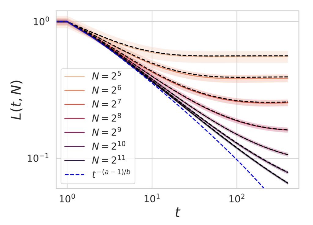
Many works have observed that the early training-time dynamics of networks with width $N$ deviates from the infinite $N$ limit with a scaling rate of $1/N$^12-14, but that after a long amount of training on sufficient quantities of data the convergence rate exhibits a task-dependent scaling law $N^{-\alpha_N}$^13-14. Our model also exhibits a transition in the convergence rates as training takes place. Below we show the early time loss of our model at $N$ compared to our model in the $N \to \infty$ limit, seeing a $1/N$ convergence rate.

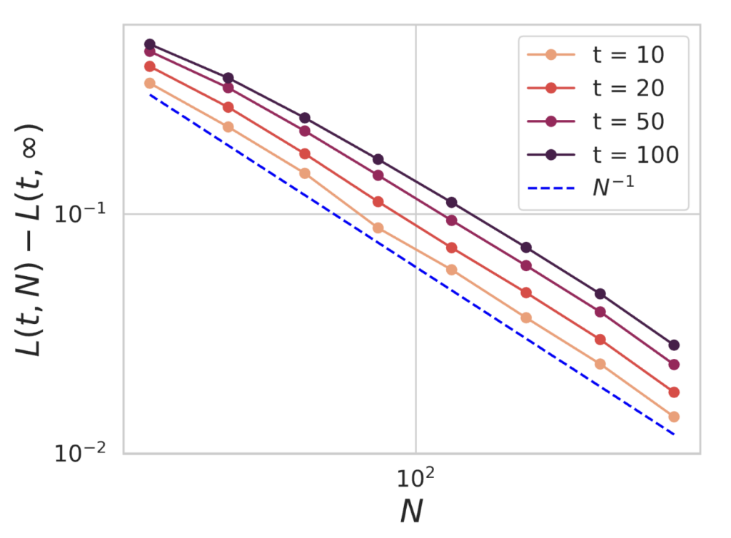
However, after significant training time, the model will eventually depend on the model size $N$ with a scaling exponent that is task-dependent (the bottleneck scaling) as we show below.

We see that this scaling law can significantly differ from the $1/N$ rate and indeed becomes task dependent.

Data Reuse and Buildup of Test/Train Loss Gaps

Many works have also observed that the early time training with a finite dataset is well approximated by training with infinite data^10-11, however over time a gap develops between training and test losses. This is also a naturally occuring feature in our model and the DMFT equations exactly describe how the test and train losses diverge over time. Below we plot dynamics for $N=512$ with varying dataset size $P$.

We note that the test and train losses are close initially but accumulate finite $P$ corrections that drive the separation of test and train. These corrections are larger for small $P$ and vanish as $P \to \infty$.

Ensembling Often Outperformed by Increasing Width

Finite sized models with random initial weights can be thought of noisy approximations of infinitely sized neural networks. This extra noise can lead to worse performance and can be eliminated by training multiple models with independent initialization in parallel and averaging their outputs, a procedure known as ensembling. However recent experiments have demonstrated that the benefits to ensembling, while non-negligible, are not as significant as the benefit of increasing model size^12-13.

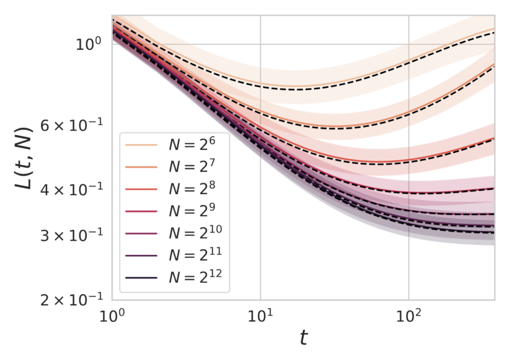
In our toy model, we can analyze the effect of ensembling on the test loss and ask whether ensembling is compute optimal. Training an ensemble of $E$ networks and averaging their outputs would incur a compute cost of $C = E N t$. Below we plot loss as a function of compute for $E=1$ and $E=4$ ensembles for varying width $N$.

At each value of compute $C$, it is prefereable to choose the larger model with $E=1$ than to use a smaller model with $E=4$. We argue the reason for this is that doubling $N$ has a similar effect on the variance as doubling $E$. However, doubling $N$ also reduces the bias.

Bias and Mode Errors

To give a flavor of how this theory works, we show how DMFT recovers the bias along the $k$th feature for all $k$. This error is given by: $$ H_k(t) = \frac{\mathbb{E}_{x} [(y(x) – f(x,t)) \psi_k(x)] }{\mathbb{E}_{x} [y(x) \psi_k(x)]}$$

Our theory explictly calculates the Fourier transform $\mathcal H_k(\omega)$ in closed form. This is given in terms of the eigenvalues $\lambda_k$, the dataset size $P$ and the model size $N$. An example of the closed form solution for the $H_k(t)$ is plotted below with $N = 128$ and varying values for $P$.

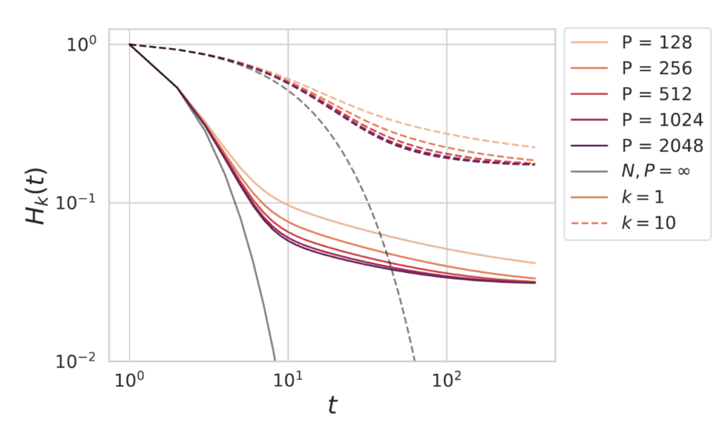
The error along the $k$-th eigendirection deviates from the infinite data and infinite model limit (gray lines) and eventually saturates as $t \to \infty$, giving a final loss which depends on $N$ and $P$. Even if $P \to \infty$, the $H_k$ curves saturate in this plot due to the finite value of $N = 128$. We show the losses for $k=1$ (solid) and $k=10$ (dashed). We find that the bias, which is set by $H_k$ decreases as $N,P$ and $t$ increase.

One Pass SGD and Batch Noise

We can also use our methods to analyze stochastic gradient descent (SGD) in discrete time without data reuse. In this setting, the finite model size and finite training time can still limit performance, but the finite batch size $B$ only introduces additional variance in the dynamics as we illustrate below. On the left, we vary the model size $N$ with batchsize set to $B=32$ and see that we still obtain model size bottlenecks which are qualitatively similar to before. We also see additional small fluctuations in the loss from batch to batch. On the right, we show $N=256$ with varying batch size, showing that the expected loss and scale of fluctuations are higher for smaller batches.

In this setting, a test-train gap is not possible since every fresh batch of data gives an unbiased estimate of the population loss. As a consequence, online learning does not experience a data bottleneck in the bias, but only additional variance from the fluctuations in the SGD updates. These updates disappear in the continuous time (infinitesimal learning rate) limit which recovers the infinite data $P \to \infty$ limit of the previously discussed gradient flow equations.

What is Missing? Feature Learning Scaling Laws

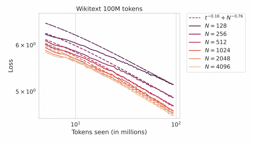
Our model is based on a kernel approximation of neural network training which fails to capture the benefits to performance due to feature learning. Below we plot neural networks trained in the kernel regime (solid) and the predicted compute scaling exponent (blue), obtained from fitting the exponents $a$ and $b$ to the measured initial kernel spectra. We also plot the loss curves for networks in the feature learning regime (dotted lines).

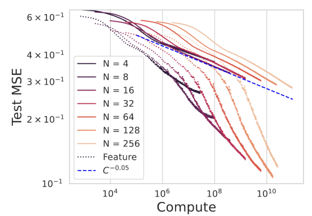
While the networks operating in the kernel regime (solid) are well described by our theoretical prediction for the compute scaling law, the networks in the rich, feature learning regime have a much better dependence on compute $C$. This illustrates that quantitatively capturing the compute optimal scaling exponents observed in practice will require a theory of how feature learning accelerates convergence during training.

Conclusion

We proposed a simple linear model to analyze dynamical neural scaling laws. This model captures many of the observed phenomena related to network training and test loss dynamics. Looking forward, theories which incorporate feature learning into the network training dynamics will improve our understanding of scaling laws. The fact that infinite sized models perform the best suggests that starting with theories of feature learning at infinite width are a good place to start.

References

1. Jared Kaplan, Sam McCandlish, Tom Henighan, Tom B Brown, Benjamin Chess, Rewon Child, Scott Gray, Alec Radford, Jeffrey Wu, and Dario Amodei. Scaling laws for neural language models. arXiv preprint arXiv:2001.08361, 2020.[↩]
2. Tom Brown, Benjamin Mann, Nick Ryder, Melanie Subbiah, Jared D Kaplan, Prafulla Dhariwal, Arvind Neelakantan, Pranav Shyam, Girish Sastry, Amanda Askell, et al. Language models are few-shot learners. Advances in neural information processing systems, 33:1877–1901, 2020.[↩]
3. Jordan Hoffmann, Sebastian Borgeaud, Arthur Mensch, Elena Buchatskaya, Trevor Cai, Eliza Rutherford, Diego de Las Casas, Lisa Anne Hendricks, Johannes Welbl, Aidan Clark, et al. Training compute-optimal large language models. arXiv preprint arXiv:2203.15556, 2022.[↩]
4. Gemini Team Google. Gemini: A Family of Highly Capable Multimodal Models, arXiv preprint arXiv:2203.15556, 2024.[↩]
5. Tamay Besiroglu, Ege Erdil, Matthew Barnett and Josh You. Chinchilla Scaling: A replication attempt. arXiv preprint arXiv:2404.10102, 2024.[↩]
6. Josh Achiam, Steven Adler, Sandhini Agarwal, Lama Ahmad, Ilge Akkaya, Florencia Leoni Aleman, Diogo Almeida, Janko Altenschmidt, Sam Altman, Shyamal Anadkat, et al. Gpt-4 technical report. arXiv preprint arXiv:2303.08774, 2023.[↩]
7. Blake Bordelon, Alex Atanasov, Cengiz Pehlevan. Dynamical Model of Neural Scaling Laws. To appear International Conference of Machine Learning 2024.[↩]
8. Elliot Paquette, Courtney Paquette, Lechao Xiao, Jeffrey Pennington. 4+3 Phases of Compute-Optimal Neural Sclaing Laws. arXiv preprint arXiv:2405.15074, 2024.[↩]
9. Licong Lin, Jingfeng Wu, Sham M. Kakade, Peter L. Bartlett, Jason D. Lee. Scaling Laws in Linear Regression: Compute, Parameters, and Data. arXiv preprint arXiv:2406:08466, 2024.[↩]
10. Preetum Nakkiran, Behnam Neyshabur, and Hanie Sedghi. The deep bootstrap framework: Good online learners are good offline generalizers. International Conference on Learning Representations, 2021[↩]
11. Niklas Muennighoff, Alexander Rush, Boaz Barak, Teven Le Scao, Aleksandra Piktus, Nouamane Tazi, Sampo Pyysalo, Thomas Wolf, and Colin Raffel. Scaling data-constrained language models. Advances in Neural Information Processing systems, 2023[↩]
12. Blake Bordelon and Cengiz Pehlevan. Dynamics of finite width kernel and prediction fluctuations in mean field neural networks. Advances in Neural Information Processing Systems, 2023.[↩]
13. Nikhil Vyas, Alexander Atanasov, Blake Bordelon, Depen Morwani, Sabarish Sainathan, and Cengiz Pehlevan. Feature-learning networks are consistent across widths at realistic scales, Advances in Neural Information Processing Systems 2023.[↩]
14. Yasaman Bahri, Ethan Dyer, Jared Kaplan, Jaehoon Lee, and Utkarsh Sharma. Explaining neural scaling laws. arXiv preprint arXiv:2102.06701, 2021.[↩]
15. Alexander Maloney, Daniel Roberts, James Sully. A solvable model of neural scaling laws. arXiv preprint arXiv:2210.16859. 2022.[↩]
16. Alexander Atanasov, Blake Bordelon, Sabarish Sainathan, Cengiz Pehlevan. Onset of Variance-limited Behavior for networks in the lazy and rich regimes. arXiv preprint arXiv:2212.12147. 2022.[↩]
17. Blake Bordelon, Abdulkadir Canatar, and Cengiz Pehlevan. Spectrum dependent learning curves in kernel regression and wide neural networks. In International Conference on Machine Learning, pp. 1024–1034. PMLR, 2020.[↩]