Infinite Limits of Neural Networks

Authors’ note: Papers discussed in this post include “Feature Learning Networks are Consistent Across Widths at Realistic Scales” coauthored by Nikhil Vyas (equal first author), Depen Morwani, and Sabarish Sainathan; and “Depthwise Hyperparameter Transfer: Dynamics and Scaling Limit” coauthored by Lorenzo Noci (equal first author), Mufan Bill Li, and Boris Hanin.

The performance of deep learning models improves with model size and dataset size in remarkably regular and predictable ways ^[1][2]. However, less is known about what kind of limiting behavior these models approach as their model size and dataset size approaches infinity. In this blog post, we aim to give the reader a relatively accessible introduction to various infinite parameter limits of neural networks. Beyond this, we aim to answer a pressing question of whether these theoretical limits actually translate to anything practically meaningful. Are large-scale language and vision models anywhere near these infinite limits? If not, in what ways do they differ?

In studying very wide and deep networks, a crucial role will be played by the parameterization of the network. A parameterization is a rule for going from a given size network to a wider (or deeper) one. More technically, it is defined by how width and depth enter when one defines the initialization, forward pass, and gradient update step of the network. Different parameterizations can lead to very different behavior as networks are scaled up.

TL;DR: Conventional parameterizations lead to neural networks performing worse with increasing depth or width. However, there are special parameterizations where performance monotonically improves as width and depth increase. These special parameterizations also keep the optimal hyperparmeters relatively stable as networks are scaled up. The key property of these parameterizations is that the network continues to learn features from the data as width an depth increase. In conventional parameterizations, very wide and deep networks are limited in their ability to learn features.

Contrasting Two Types of Infinite Width Limit

Below, we train CNNs of varying channel count for a few epochs on the CIFAR-10 image classification task. We will call the channel count the width and denote it by $N$. We start with a width 64 network (solid), and increase the width according to the commonly used NTK parameterization (dashed). This parameterization will be precisely defined in the next section. We keep all other hyperparameters fixed. As the model size increases, the test loss gets worse.

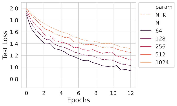
Do wider models inherently train slower and generalize worse? Such a finding would be quite inconsistent with the recent results of larger language and vision models achieving top performance.

Actually, this effect is entirely an artifact of the parameterization. When using the same architecture in another parameterization known as the maximal update parameterization or $\mu$P for short (solid lines below), we find that increasing the width $N$ leads to improved performance. We will precisely define this parameterization later on.

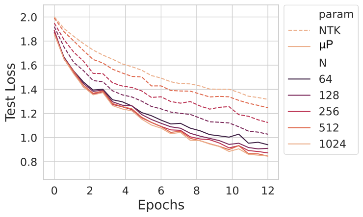
Here that we have set up things so that the width 64 network has identical dynamics in both paramterizations, and the other networks are scaled up from that one using either NTK or $\mu$P parameterizations.

What is different between these two parameterizations? Why does one give similar training dynamics across model sizes while the other does not? To understand the difference, we need to investigate their limiting behaviors as width becomes larger. Mathematically, this means studying the limit $N \to \infty$.

Limit 1: Neural Tangent Kernel (NTK)

Depending on the architecture of a given network, the width of a given layer is either: the feedforward dimension in a dense layer, the number of channels in a convolutional layer, the size of the residual stream, or the dimenson of the keys and queries for each attention head. Infinite width limits usually mean that we take this hidden dimension to infinity in each layer of the network.

For simplicity, we focus on a dense feedforward neural network, though we stress that these ideas can straightforwardly be extended to other architectures (convnets, resnets, transformers, state space models).

We initialize all weights to be drawn from the unit Gaussian $\mathcal N(0, 1)$, although any well-behaved¹ distribution with mean 0 and variance 1 will lead to the same results. We take the depth to be $L$. For each layer $\ell \in {1, \dots L }$, the entries of the hidden layer “preactivation” vector $\mathbf h^\ell$ are given by

$$h^{\ell+1}_i(\mathbf x) = \frac{1}{\sqrt{n_{\ell}}} \sum_{j} W_{ij}^{\ell+1} \varphi(h^{\ell}_j(\mathbf x)), \quad h^1_i(\mathbf x) = \frac{1}{\sqrt{n_0}} \sum_j W_{ij}^1 x_j,$$

where $\varphi$ is a nonlinearity acting element-wise, and $n_{\ell}$ is the width of layer $\ell$ and $n_0$ is the dimension of the inputs. The output of the network is then given by the last layer:
$$f(\mathbf x; \mathbf W) = h^{L}(\mathbf x).$$

Going forward, we will take all widths $n_\ell = N$. The factors of $1/\sqrt{n_\ell}$ at each layer are there so that (by the central limit theorem) each $h_{i}^\ell$ is $\Theta_N(1)$ in size². This allows for the network output to be finite in the limit of $N \to \infty,$ and for the network to be trainable.

In this parameterization, the weights and preactivations move during gradient descent by:

$$\Delta W_{ij}^\ell \sim \Theta(N^{-1}) \ , \ \Delta h_i^\ell \sim \Theta(N^{-1/2}).$$

We note that in the $N \to \infty$ limit, because the preactivations do not change, the hidden representations of the network will be static during training. The network not will learn internal representations of the data.

Because the weights move only infinitesimally as $N\to \infty$, the model behaves like its linearization in weight space. This gives a linear model (also called a kernel method). This is the neural tangent kernel (NTK)³.

One can successfully study the training and generalization of sufficiently wide neural networks by studying this linear model. Our group’s prior work ^[3][4] gives exact analytic equations for the learning curves in this infinite width limit, using methods in statistical physics and random matrix theory. See also our group’s recent work ^[5] for an accessible overview of these ideas. One can also study the training dynamics of linear models, and recover many of the empirical phenomena observed in large scale language and vision models – see our next blog post!

Limit 2: Feature-Learning Infinite Width Limit (µP)

Unfortunately, by their very definition, linear models do not learn features. Feature learning is widely belived to be responsible for the impressive performance of deep learning. Further, in networks that learn features, wider models empirically tend to perform better. The NTK parameterization does not capture these phenomena – luckily, there is an alternative parameterization that does.

The aim is to parameterize the network so that it can learn features even at infinite width. This has been studied under the name mean field paramerization for two layer networks ^[6][7] and generalized to arbitrary architectures by Yang et al ^[8] under the name maximal update parameterization, commonly abbreviated as $\mu$P. A characterization of the infinite width limit using dynamical mean field theory was done by our group in ^[9].

The $\alpha$ Parameter

A simple way to derive this parameterization is to slightly modify the above feedforward network by adding a single additional (non-trainable) parameter $\alpha$ to the very last stage of the forward pass, as done in ^[10]:

$$f_\alpha(\mathbf x; \, {\mathbf W^\ell}_{\ell}) = \alpha \, h^{L}(\mathbf x).$$

Although this modification appears relatively innocuous, it substantially impacts the amount by which the network deviates from being a linear model. When $\alpha$ is very large, relatively small changes in the weights can lead to large changes in the output $f_\alpha$. The model is then well-approximated by its weight space linearization. This is called the lazy limit, kernel limit, or lazy training. Therefore at large $\alpha$, the network does not learn features.

By contrast, small $\alpha$ networks need to significantly change their weights to induce the necessary change in the output ^[10][11][12]. This is called the rich regime and allows for the network to learn features.

In order to keep the gradients from exploding or vanishing, one needs to scale the learning rate⁴ as $\eta \sim \alpha^{-2}$. Then, in each step of gradient descent one can show that the changes of the preactivations go as:

$$\Delta h_i^\ell \sim \frac{\eta\, \alpha}{\sqrt{N}} \sim \frac{1}{\alpha \sqrt{N}}.$$

We see that choosing $\alpha = 1/\sqrt{N}$ causes $\Delta h_i^\ell$ to remain order $1$ even as $N \to \infty$. This allows for feature learning at infinite width while keeping the network trainable. This is exactly the rescaling required to achieve $\mu$P.

The Infinite Width Feature Learning Limit

The $N \to \infty$ limit gives a dynamical system for preactivations $\mathbf h^\ell$ which can be characterized using a method from statistical physics, known as dynamical mean field theory (DMFT) ^[13]. Below we show a figure from that paper. We plot the correlation between preactivations $\mathbf x^\mu, \mathbf x^\nu$ across different layers $\ell$. $H^{\ell}_{\mu\nu} = \frac{1}{N} \mathbf h^\ell(x_\mu) \cdot \mathbf{h}^\ell(x_\nu)$ for pairs of samples $\mathbf x_\mu, \mathbf x_\nu$ across different layers $\ell \in \{1,…,5\}$ after training.

The architecture and dataset is just a linear neural network learning the first two classes of CIFAR. Despite this simple setting, already we see that the DMFT solution captures the network’s ability to learn features while the NTK limit cannot.

Convergence to the Feature Learning Limit

We have described two different infinite width limits of neural networks. From the point of view of a practitioner, what really matters is whether such limits are descriptive of realistic large models. We investigate this question empirically in our recent paper ^[14]. We find that $\mu$P networks approach their infinite width behavior at the scales used in practice, by contrast to NTK-parameterized networks.

We look at CNNs trained on vision tasks with millions of training examples (CIFAR-5M and ImageNet) as well as language modeling on Wikitext-103. We vary the width of models parametrized in $\mu$P so that they approach a well-defined feature learning limit.

Loss Curves

Below, we show that the loss dynamics for networks of varying width $N$ in $\mu$P all begin to coincide at sufficiently large $N$.

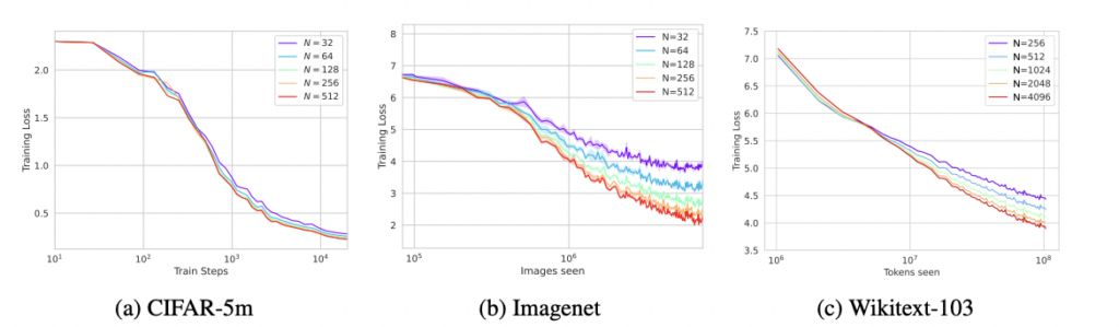
We also note that, unlike in NTK parameterization, the wider models tend to outperform the narrower models, similar to observations in ^[15].

Individual Logits

Not only do the loss curves begin to coincide past a given width, but even the individual logit outputs for any fixed held-out test point begin to agree at large $N$. Plotted below is the output of the network on the correct logit for a vision and language modeling task in $\mu$P. We use a single (randomly selected) test point in each case.

Learned Representations

Another prediction of the DMFT treatment is that for wide enough networks, the learned internal representations will converge to the same limiting values. We indeed observe this in practice. Below we plot the preactivations and final-layer feature kernels for a ResNet on CIFAR-5m, and observe that the network learns the exact same representations across different widths. We also plot the feedforward preactivation histograms, as well as attention weights for a transformer trained on language modeling of Wikitext-103. For more quantitative measures of this convergence, see our paper.

Finite Width Corrections

One can ask what role finite width plays in deviating a network from its infinite-width NTK or $\mu$P limit. There are two primary effects to the dynamics of finite width networks compared to the infinite width networks. First, finite networks exhibit dependence on their precise initialization of parameters which infinite networks do not. This can be thought of as additional variance in the model. This variance can be eliminated by averaging network outputs over different random initializations. This is known as ensembling. However, even after ensembling, finite models are still biased compared to infinite width models.

Fine-grained bias variance decompositions

To measure how large the variance correction and bias correction of finite width models are, we ensemble several randomly initialized networks. Below, we plot the average loss of single models of varying width in solid lines and their ensemble averaged loss in dashed lines. Although ensembling is helpful, going wider still is better than ensembling.

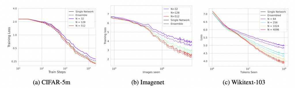
These results indicate that bias corrections in the dynamics tend to dominate the gap between finite and infinite models.

For a deeper theoretical study of these finite-width effects, see our prior works ^[16][17]. See also our follow up blog post and recent paper ^[18] for a solvable model of this and its implications on the compute-optimal allocation of resources.

Practical Benefit: Hyperparameter Transfer Across Widths and Depths

Because the training dynamics of $\mu$P become consistent across widths, one can perform hyperparameter search on smaller models to find the optimal hyperparameters (e.g. learning rate, momentum, etc). One then scales the width up and sees that those hyperparameters remain nearly optimal for the wider networks. See ^[15] for details. This offers large potential savings of compute time when training large scale models.

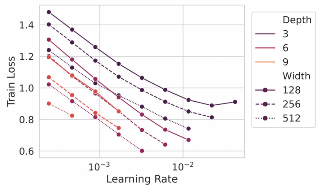
Optimal hyperparameters are not stable across widths in most parameterizations. For example, in standard (Pytorch default) parameterization, learning rates do not transfer over either width or depth – as we show below.

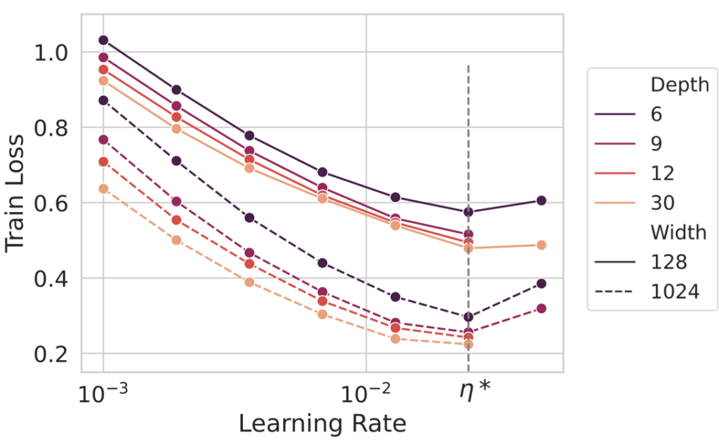
Recently, our paper ^[19] as well as concurrent work ^[20] has extended this to allow for hyperparameter transfer across both widths and depths. Below we show an example of the loss as a function of learning rate for various sized models, showing that the optimum is essentially constant across different sizes.

The key philosophy to obtain this hyperparameter transfer is to design a parameterization where the model converges to a well-defined limit and maintains the same rate of feature learning across all network sizes.

Conclusion

We have introduced two distinct parameterizations of neural networks that allow for infinite width limits to be taken. The NTK parameterization gives rise to a linear model at infinite width. This linear model does not learn features and therefore fails to capture crucial aspects of deep learning. The maximal update parameterization $\mu$P on the other hand gives a feature-learning limit that performs well and is representative of realistic wide networks. We observed consistent dynamics even at modest and realistically-accessible widths, indicating that networks were approaching that limit. We’ve commented on the applications of this for studying learned representations and transferring hyperparameters across widths and depths. We believe that infinite-width feature learning networks have much to offer both theorists and practitioners.

While the infinite width and depth models tend to perform best, it is important to know the scaling behavior of the loss as a function of training time and model size in order to optimally allocate compute resources. Check out our follow-up blog post that gives a solveable model of these scaling laws.

Footnotes

¹ That is, any distribution with finite moments, e.g. a uniform distribution. [Return to text ↩]

² Here we will use $O_N(1)$ to denote that the quantity remains constant as $N$ is varied. We will also use $\Theta(f(N))$ to denote that a given quantity as a function of $N$ can be bounded from both above and below by (appropriate constants) times the function $f(N)$ as $N \to \infty$. That is, it has the same asymptotic behavior as $f(N)$. [Return to text ↩]Return to text

³ In the infinite-width limit, the kernel turns out to be independent of the initialization $\mathbf W_0$. This is an important fact, as the leading correction of finite-width is to introduce a dependence on initialization to the kernel that can be viewed as a source of noise or “variance” that hurts performance. [Return to text ↩]

⁴ This learning rate scaling follows from the fact that the NTK goes as $\partial_\theta f \cdot \partial_\theta f \sim O(\alpha^2)$ and the learning rate should be scaled inversely with the max eigenvalue of the kernel. [Return to text ↩]

References

1. Kaplan, J., McCandlish, S., Henighan, T., Brown, T.B., Chess, B., Child, R., Gray, S., Radford, A., Wu, J. and Amodei, D., 2020. Scaling laws for neural language models. arXiv preprint arXiv:2001.08361.[↩]
2. Hoffmann, J., Borgeaud, S., Mensch, A., Buchatskaya, E., Cai, T., Rutherford, E., Casas, D.D.L., Hendricks, L.A., Welbl, J., Clark, A. and Hennigan, T., 2022. Training compute-optimal large language models. arXiv preprint arXiv:2203.15556.[↩]
3. Bordelon, B., Canatar, A. and Pehlevan, C., 2020, November. Spectrum dependent learning curves in kernel regression and wide neural networks. In International Conference on Machine Learning (pp. 1024-1034). PMLR.[↩]
4. Canatar, A., Bordelon, B. and Pehlevan, C., 2021. Spectral bias and task-model alignment explain generalization in kernel regression and infinitely wide neural networks. Nature communications, 12(1), p.2914.[↩]
5. Atanasov, A., Zavatone-Veth, J. and Pehlevan, C., 2024. Scaling and renormalization in high-dimensional regression. arXiv preprint. https://arxiv.org/abs/2405.00592.[↩]
6. Mei, S., Montanari, A. and Nguyen, P.M., 2018. A mean field view of the landscape of two-layer neural networks. Proceedings of the National Academy of Sciences, 115(33), pp.E7665-E7671.[↩]
7. Rotskoff, G.M. and Vanden-Eijnden, E., 2018. Neural networks as interacting particle systems: Asymptotic convexity of the loss landscape and universal scaling of the approximation error. stat, 1050, p.22.[↩]
8. Yang, G. and Hu, E.J., 2021, July. Tensor programs iv: Feature learning in infinite-width neural networks. In International Conference on Machine Learning (pp. 11727-11737). PMLR.[↩]
9. Bordelon, B. and Pehlevan, C., 2022. Self-consistent dynamical field theory of kernel evolution in wide neural networks. Advances in Neural Information Processing Systems, 35, pp.32240-32256.[↩]
10. Chizat, L., Oyallon, E. and Bach, F., 2019. On lazy training in differentiable programming. Advances in neural information processing systems, 32.[↩][↩]
11. Geiger, M., Spigler, S., Jacot, A. and Wyart, M., 2020. Disentangling feature and lazy training in deep neural networks. Journal of Statistical Mechanics: Theory and Experiment, 2020(11), p.113301.[↩]
12. Woodworth, B., Gunasekar, S., Lee, J.D., Moroshko, E., Savarese, P., Golan, I., Soudry, D. and Srebro, N., 2020, July. Kernel and rich regimes in overparametrized models. In Conference on Learning Theory (pp. 3635-3673). PMLR.[↩]
13. Bordelon, B. and Pehlevan, C., 2022. Self-consistent dynamical field theory of kernel evolution in wide neural networks. Advances in Neural Information Processing Systems, 35, pp.32240-32256[↩]
14. Vyas, N., Atanasov, A., Bordelon, B., Morwani, D., Sainathan, S. and Pehlevan, C., 2024. Feature-learning networks are consistent across widths at realistic scales. Advances in Neural Information Processing Systems, 36.[↩]
15. Yang, G., Hu, E.J., Babuschkin, I., Sidor, S., Liu, X., Farhi, D., Ryder, N., Pachocki, J., Chen, W. and Gao, J., 2022. Tensor programs v: Tuning large neural networks via zero-shot hyperparameter transfer. arXiv preprint arXiv:2203.03466.[↩][↩]
16. Atanasov, A., Bordelon, B., Sainathan, S. and Pehlevan, C., 2022, September. The Onset of Variance-Limited Behavior for Networks in the Lazy and Rich Regimes. In The Eleventh International Conference on Learning Representations.[↩]
17. Bordelon, B. and Pehlevan, C., 2024. Dynamics of finite width kernel and prediction fluctuations in mean field neural networks. Advances in Neural Information Processing Systems, 36.[↩]
18. Bordelon, B., Atanasov, A. and Pehlevan, C., 2024. A Dynamical Model of Neural Scaling Laws. arXiv preprint arXiv:2402.01092.[↩]
19. Bordelon, B., Noci, L., Li, M.B., Hanin, B. and Pehlevan, C., 2023, October. Depthwise Hyperparameter Transfer in Residual Networks: Dynamics and Scaling Limit. In The Twelfth International Conference on Learning Representations.[↩]
20. Yang, G., Yu, D., Zhu, C. and Hayou, S., 2023. Tensor programs vi: Feature learning in infinite-depth neural networks. arXiv preprint arXiv:2310.02244.[↩]