The Hidden Linear Structure in Diffusion Models and its Application in Analytical Teleportation

Diffusion models are powerful generative frameworks that iteratively denoise white noise into structured data via learned score functions. Through theory and experiments, we demonstrate that these score functions are dominated by a linear Gaussian component. This finding unlocks closed-form sampling trajectories, explains coarse-to-fine feature emergence and enables analytical teleportation to skip 20–30% of early steps without quality loss.

Why study diffusion models?

Diffusion models—and their close relatives, flow matching models—have rapidly become the workhorses of modern generative AI, powering state-of-the-art image (e.g. Stable Diffusion), audio, video (e.g. Sora), and protein synthesis (e.g. AlphaFold 3). These models generate samples via an iterative denoising process that gradually transforms pure noise into richly structured data. At its core, a neural network is trained to denoise, once trained, it approximates the score function—the gradient of the noise-smoothed data density—and following this vector field guides samples toward regions of high data likelihood.

Despite the remarkable practical success of diffusion models, key conceptual issues persist:

1. Relation between noise and sample. How does the model “decide” what to generate? How does the initial noise pattern determines the final sample?
2. Feature emergence. At what stages of the sampling process are different features—such as coarse layout versus fine details—established?
3. Generalization vs. memorization. Do diffusion networks memorize the training data (i.e., learn a mixture of delta functions), if not, how do they exhibit creativity and generalize beyond what they’ve seen?

Admittedly, these questions are challenging: how can we truly understand a deep neural network trained through a complex optimization process on natural datasets? Here, we adopt a normative perspective to address these issues, asking how neural networks should behave if they optimally minimize the loss for a given data distribution. For diffusion models, optimality implies accurately learning the true score function $\nabla \log p(x)$ of the distribution. So we analyze the analytical scores of various tractable distributions approximating the real data—including Gaussian and Gaussian mixture models (GMMs)—and compare these analytical scores directly with those learned by neural networks.

Out central—and at first surprising—claim is:

For moderate to high noise levels, the learned score vector of diffusion models is dominated by the linear score of Gaussian
$$s_{\rm Gauss}(x;\sigma) \;=\; (\Sigma + \sigma^2 I)^{-1}(\mu – x)\,$$
where $\mu$ and $\Sigma$ are the mean and covariance of training data. ^[1]

This Gaussian score approximation extends far beyond the anticipated “far-field” regime, remaining valid deeper into the sampling process than naive theory would predict—opening up both theoretical insights and practical opportunities for acceleration.

1. The Linear Score of Gaussian Model: Exact Solutions and Intuition

1.1 From data covariance to closed-form trajectories

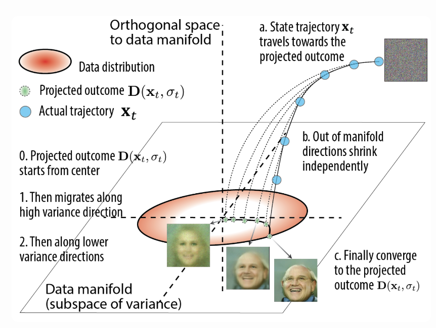
If the dataset were truly Gaussian, then its score function would exactly be a linear vector field. Consequently, the sampling equation—known as the Probability Flow ODE—simplifies to a linear, time-varying ordinary differential equation (ODE) that admits a closed-form solution. By decomposing the covariance $\Sigma = U\,\mathrm{diag}(\lambda_k)\,U^T$, we find that the state $x_t$ evolves independently along each principal component $u_k$:
$$
x_t = \mu
\;+\; \sum_{k=1}^r \underbrace{\sqrt{\tfrac{\sigma_t^2 + \lambda_k}{\sigma_T^2 + \lambda_k}}}_{\psi(t,\lambda_k)} \,\bigl[u_k^T(x_T-\mu)\bigr]\,u_k
\;+\;\underbrace{\frac{\sigma_t}{\sigma_T} \ x^{\perp}_T}_{\text{off-manifold shrinkage}}.
$$
At the same time, the denoised images $\mathbf D(x_t,\sigma_t)$ will follow on-manifold dynamics, moving along PC in descending order of variance
$$
\mathbf D(x_t,\sigma_t) = \mu
\;+\; \sum_{k=1}^r \underbrace{\tfrac{\lambda_k}{\sqrt{(\lambda_k + \sigma_t^2)(\lambda_k + \sigma_T^2)}}}_{\xi(t,\lambda_k)} \,\bigl[u_k^T(x_T-\mu)\bigr]\,u_k
.
$$

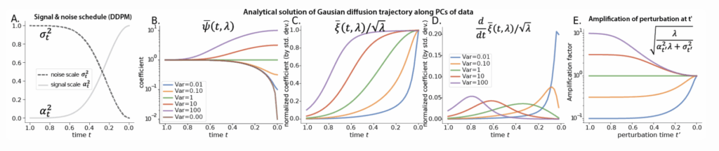
Figure 1: The analytical solution to sample generation dynamics for the Gaussian model, using variance preserving (e.g. DDPM) convention: A. The noise and signal schedule σ and α from ddpm-CIFAR-10; B. Special function ψ governs the dynamics of state along each principal axis; C. Special function ξ governs the dynamics of the denoiser output along each PC, normalized by the standard deviation of PC; D. Time derivative of special function ξ in C., highlighting the “critical period” when each feature develops most rapidly; E. The special function which quantifies the amplification effect of a perturbation along PC k at time t’; In B.C.D.E. consistent color scheme shows the eigenmode from high to low variance.

1.2 Interpretation and qualitative validation

Some immediate insights follow:

• Feature ordering. The state and denoiser evolves most rapidly along each direction 𝑢 𝑘 , when the noise variance 𝜎 𝑡 2 matches the signal variance 𝜆 𝑘 . Thus, high-variance (coarse, layout) features are determined early in reverse diffusion, and low-variance (fine, textury) details are determined later.
• Veil of noise. Since the noise corresponds to the lowest variance (off-manifold) component, it will be removed at the very end. Thus, although most visual features are determined earlier in the process, they become clearly visible only once the veil of noise is finally lifted.
• Trajectory geometry. We show that the state 𝑥 𝑡 moves approximately along a 2D “rotation” in the plane spanned by its starting 𝑥 𝑇 and final state 𝑥 0 , with only small corrections in the middle. This explains why sampling paths in high-dimensional diffusion models (e.g. Stable Diffusion) empirically lie in low-dimensional (often 2d) subspaces.

• Noise to image mapping. This solution gives us the explicit relationship between the initial noise $x_T$ and the final images $x_0$, in a formula also known as Wiener Filter. The amount of feature at final sample (location along $u_k$ axis) is determined by the subtle alignment of the initial noise pattern with that feature $u_k^T(x_T-\mu)$ and the amplification factor $\psi(0,\lambda_k)$. Thus features in the final samples already have minimal root in the initial noise.
• Perturbation sensitivity. For a linear dynamical system, sensitivity analysis allows one to analytically predict how a perturbation at time $t’$ influence the final sample $x_0$. We found perturbations along a direction of variance $\lambda$ at time $t^{‘}$ are amplified by a factor $\sqrt{\tfrac{\lambda}{\sigma_{t’}^2 + \lambda}}$, which is largest when $\sigma_{t’}^2 \ll \lambda$. This explains the prior observation that early noise injections alter “layout” while late noise injections tweak “texture” (DDPM, 2020).

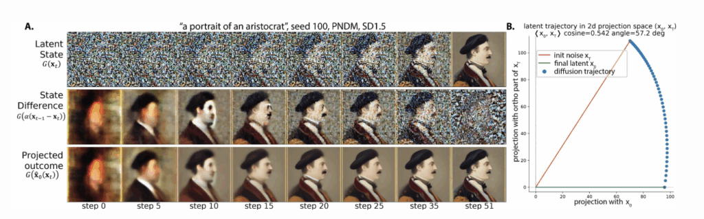
Figure 3: Qualitative aspects of Stable Diffusion’s sampling process that are consistent with Gaussian theory A. Trajectories of states (top row), scaled differences between nearby states (middle row), and denoiser/projected outcome (bottom row). G denotes Stable Diffusion’s VAE decoder, which converts latent states to images. B. Trajectory of x_t projected onto the plane spanned by x_T and x_0. Trajectories are effectively two-dimensional and resemble a rotation from x_T to x_0. Both feature-emergence order and the low dimensionality of these trajectories align with predictions from the Gaussian model.

2. Theory Meets Practice: When “Far-Field” Holds

The theory of Gaussian scores is elegant, but how is it relevant to actual diffusion models, given that distributions worth modeling are usually far from Gaussian? Here, we consolidate this connection both theoretically and empirically.

2.1 Theory: Multipole-style expansion

Intuitively, when enough noise has been added to the data, the resulting distribution should become Gaussian. More formally, we show that for any bounded point cloud, when the noise scale $\sigma$ far exceeds the cloud’s radius (i.e. trace of covariance $\Sigma$), a multipole-like expansion reveals that the exact score of the point cloud matches, to the first order, that of a Gaussian with identical mean and covariance. $$ s_{\rm true}(x;\sigma)\;=\;\nabla\log p(x;\sigma) \;\approx\; (\Sigma+\sigma^2I)^{-1}(\mu-x) $$ In physics, this mirrors how a distant charge distribution “blurs” into a point charge (plus dipole, etc.) at long range. Analogously, if you stand at the edge of the galaxy, aiming at a particular point on Earth is essentially the same as aiming at Earth’s center—differences only emerge when you are closer.

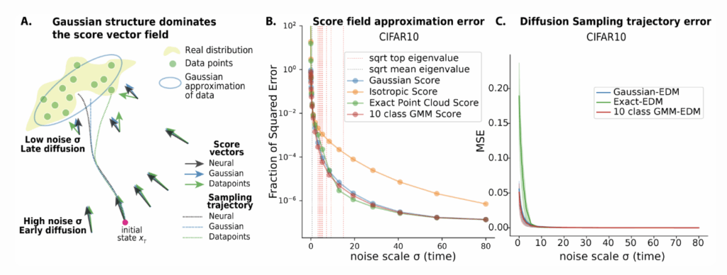
2.2 Empirical Score Comparisons: Far-field dominated by Gaussian

Using three natural image datasets (CIFAR-10, FFHQ64, AFHQv2-64), we evaluate the difference between,

• Neural scores $s_\theta(x,\sigma)$ from pre-trained EDM diffusion models (Karras et al., 2022)
• Analytic scores $s_{\rm analytic}(x,\sigma)$:
  • Isotropic Gaussian $(\mu-x)/\sigma^2$
  • Full Gaussian $(\Sigma+\sigma^2I)^{-1}(\mu-x)$
  • Per-class Gaussian mixture (one Gaussian per CIFAR-10 label)
  • Exact delta mixture (the true training-set score) 

We measure fraction of unexplained variance $$1 – \frac{\mathbb{E}\|s_\theta – s_{\rm analytic}\|^2}{\mathbb{E}\|s_\theta\|^2}\,.$$

Key finding: At high noise regime, $\sigma \gtrsim 1$, the Gaussian score explains > 99% variance of the neural score—nearly as well as a 10-mode mixture; at low noise regime, Gaussian score also approximates far better than the delta mixture score.

3. Early Sampling Dynamics Well Predicted by Gaussian

If the scores match, do sampling trajectories match? By comparing:

• The analytical solution to Gaussian ODE,
• A 2nd-order Heun integrator on the learned neural score, and
• A classic RK4 on mixture scores,

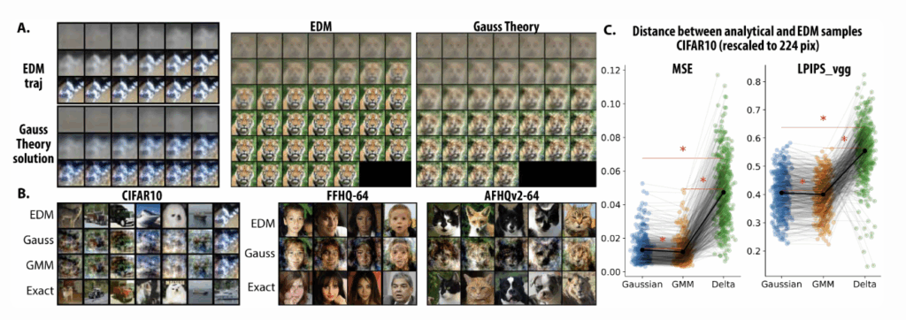
we show that the first 15–30% of sampling steps of a diffusion model are almost perfectly tracked by the Gaussian model. Beyond that point—where σ drops below the covariance’s largest eigenvalue—the approximation degrades, and the network’s true, multimodal structure takes over.

Visually, analytical samples from the Gaussian solution strikingly capture key aspects of global layout, color palettes, and shading, diverging primarily on finer textures. Quantitatively, Gaussian samples are closer (in MSE and LPIPS) to the full EDM samples than those from the exact delta score. This also suggests, what the neural network learns is closer to the Gaussian or Gaussian mixture, i.e. the aggregated data statistics, instead of memorizing exact data points.

4. Beyond a Single Gaussian: Low-Rank Mixtures

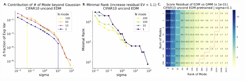
To study the low-noise regime, we fit Gaussian mixture models to the dataset with varying numbers of clusters $K$ and covariance matrices of varying rank $r$, and compared their analytical scores to the neural scores. Three central trends emerge:

1. Few clusters suffice. Even at moderate noise, going from $K=1$ to $K=10$ yields large gains in explained variance; further increases yield diminishing returns, and at very low $\sigma$, too many modes actually harm approximation (a U-shaped curve).
2. Few ranks suffice at high noise. At high $\sigma$, a very low rank covariance (e.g. $r\ll D$) suffices—small eigenvalues are drowned out by noise. As $\sigma$ decreases, the minimal needed rank climbs, tracking which principal components become “visible” when $\lambda_k \gtrsim \sigma^2$.
3. Mode-Rank trade-offs. When a single cluster was used, it required a higher-rank covariance; in contrast, when more clusters were added, each one could have a lower-rank covariance. 

Together, this paints the following picture of the data manifold: high noise submerges the signal details, so only a few PCs of the covariance are needed to predict the score; low noise reveals the intricate details of the data manifold, similar to a globally curved patchwork of locally flat geometries.

Learning Dynamics: Simpler Scores First

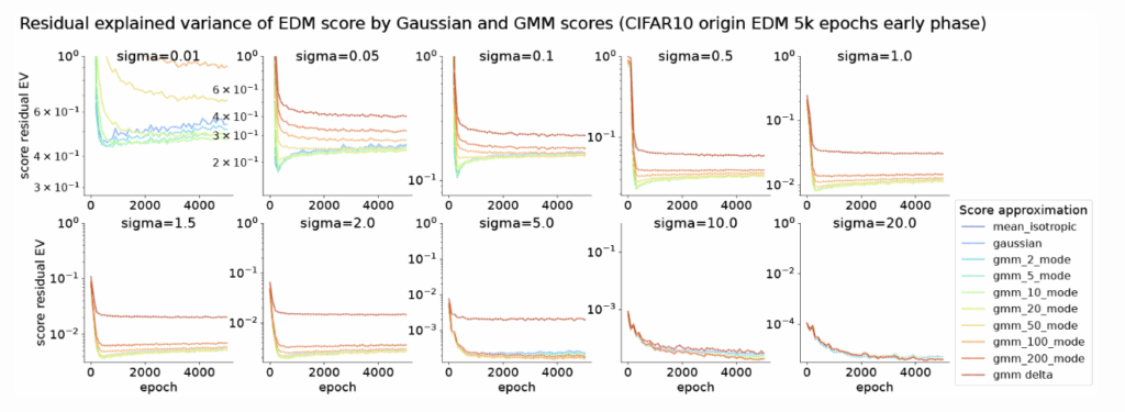
Figure 7: Learning dynamics of score neural network with idealized scores (Gaussian, Gaussian mixture, and Exact) as reference. Each panel shows a different noise scale $\sigma$ and plots residual explained variance (1 – EV) as a function of training epoch. Each line shows the residual EV of the neural score with respect to one idealized score model. At higher noise scales, all score approximators deviate negligibly from the neural score and from each other. At lower noise scales ($\sigma\leq 1.5$), the deviation between the neural score and the Gaussian score first decreases, and then increases slightly. This indicates that the neural score approaches the score of the Gaussian model before it learns additional structure.

So how does this score structure evolve during training? By checkpointing training progress on CIFAR-10, FFHQ, and MNIST, we show:

• At high noise ($\sigma\ge10$), the neural score converges towards all analytic scores (Gaussian, mixture, delta) monotonically.
• At lower noise, the neural score first aligns with the single Gaussian (and few-mode mixtures), then deviates as it learns finer structure. In contrast, its convergence to the delta mixture is monotonic and a large gap remains. 

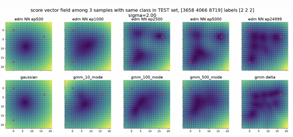
Visually, the score vector field starts as a single basin centered at the global mean and then gradually fractures into multiple basins similar to Gaussian mixture. This mirrors how a neural network first captures the coarse structure of the score field (e.g., the Gaussian approximation) before sculpting its fine details.

Analytical Teleportation: Speeding Up Sampling

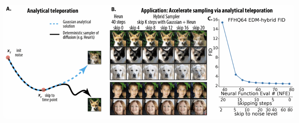
Armed with an analytical description of the initial sampling trajectory, we can “teleport” from $x_T$ directly to an intermediate $x_{t’}$, skipping a number of neural function evaluations, specifically, we:

1. Evaluate $x_{t’}$ via the closed-form Gaussian solution, using the dataset mean $\mu$ and covariance $\Sigma$.
2. Continue integrating the PF-ODE with the learned score from $t’$ to $0$. Experiments on unconditional CIFAR-10 and FFHQ64 with the Heun sampler show that we can safely skip 15–30% of steps while maintaining FID within 3% of the full sampler (achieving an unconditional CIFAR-10 FID = $1.93$ at 25 NFE). 

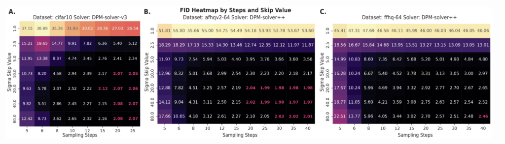
This hybrid scheme is orthogonal to other improvements on sampler (e.g. UniPC, DPM-Solver), and can be plugged in to accelerate any ODE- or SDE-based method.

Conclusion & Future Directions

Key take-homes

1. Linear scores of Gaussian are not just mathematically neat—they dominate learned diffusion scores in a wide range of noise scales.
2. This explains the outline-first, details-later nature of image synthesis, low-dimensional sampling paths, and why early perturbations shape layout while late ones sculpt texture.
3. Neural score networks learn simple (Gaussian) structure before complex (multimodal) structure, mirroring classic spectral bias.
4. Analytical teleportation offers a practical route to cut sampling time by 20-30 percent without sacrificing quality.

Since the release of our paper, we’ve been pleased to see several exciting follow-up and related developments in the field:

• Creativity and ideal score under constraints. The Gaussian score can be regarded as the optimal score given linear function constraints ^[2], so what about other constraints on the function approximator? Recent works ^[3][4] derive the ideal score under locality and equivariance constraints (related to convolutional networks), and find these “ideal” scores predict the generated images better than our Gaussian theory, highlighting the importance of inductive bias.
• Theory of diffusion learning dynamics. The existence of linear structure allows many classic learning theory tools to be applied to diffusion and have real world relevance. Recently, theoretical analysis of diffusion training dynamics in linear setting has revealed a spectral bias in distribution learning: higher-variance data dimensions are learned before lower-variance ones ^[5] mirroring the similar variance ordering in sampling.
• Reproducibility and consistency. Multiple groups observe that, despite different initializations, different architectures ^[6] or even non-overlaping data splits ^[7], large diffusion models converge to nearly identical noise-to-image mappings— potentially due to the shared Gaussian-linear component^[8]
• Antithetic noise structure: Recent work^[9] shows that negating the initial noise, $z \to -z$, produces samples with flipped attributes (e.g., white male → black female). This mirrors the Gaussian solution: flipping z reverses alignment along principal components $u_k^\top(x_T – \mu)$, yielding opposite high-level features.
• Regularity of sampling trajectory and acceleration. The low–dimensionality of diffusion’s sampling path has inspired new acceleration techniques^[10][11] that exploit this regularity to reduce sampling time further.
• Finetuning and human alignment: Surprisingly, some of our findings inspired the finetuning techniques of image or video diffusion models. Since different noise levels correspond to different types of features, we could target specific noise levels for finetuning particular features^[12]; Similarly, by injecting noise of different strength, we could create variations on different levels to obtain fine grained human preference annotation.^[13]

We hope our work inspires more normative analysis of generative models, by unveiling latent structure, we could enable faster sampling, more focused fine-tuning, and deeper insights into their creativity. 

1. In the blog post, we will stick to the so-called variance exploding (VE) or EDM convention of diffusion, where Gaussian noise is directly added to the samples without rescaling the noised sample. For the variance preserving (VP) convention, we just need to make substitutions $\mathbf{x}_t\mapsto \mathbf{x}_t/\alpha_t$ and $\sigma_t\mapsto \sigma_t/\alpha_t$, where $\sigma_t$ and $\alpha_t$ and noise and signal scale at time $t$. [↩]
2. Li, X., Dai, Y., & Qu, Q. (2024). Understanding generalizability of diffusion models requires rethinking the hidden gaussian structure. NeurIPS[↩]
3. Kamb, M., & Ganguli, S. (2024). An analytic theory of creativity in convolutional diffusion models. arXiv:2412.20292.[↩]
4. Niedoba, M., Zwartsenberg, B., Murphy, K., & Wood, F. (2024). Towards a Mechanistic Explanation of Diffusion Model Generalization. arXiv:2411.19339.[↩]
5. Wang, B., Pehlevan, C. (2025). An analytical theory of power law spectral bias in the learning dynamics of diffusion models. arXiv:2503.03206.[↩]
6. Zhang, H., Zhou, J., Lu, Y., Guo, M., Wang, P., Shen, L., & Qu, Q. (2024). The emergence of reproducibility and consistency in diffusion models. ICML.[↩]
7. Kadkhodaie, Z., Guth, F., Simoncelli, E. P., & Mallat, S. (2023). Generalization in diffusion models arises from geometry-adaptive harmonic representations. ICLR, arXiv:2310.02557.[↩]
8. Li, X., Dai, Y., & Qu, Q. (2024). Understanding generalizability of diffusion models requires rethinking the hidden gaussian structure. NeurIPS.[↩]
9. [Jia, J., Liu, S., Song, B., Yuan, W., Shen, L., & Wang, G. (2025). Antithetic Noise in Diffusion Models. arXiv:2506.06185.[↩]
10. Chen, D., Zhou, Z., Wang, C., Shen, C., & Lyu, S. (2024). On the trajectory regularity of ode-based diffusion sampling. ICML, arXiv:2405.11326.[↩]
11. Wang, G., Peng, W., Li, L., Chen, W., Cai, Y., & Su, S. (2024). Diffusion Sampling Correction via Approximately 10 Parameters. arXiv:2411.06503.[↩]
12. Yang, S., Chen, T., & Zhou, M. (2024). A dense reward view on aligning text-to-image diffusion with preference. ICML, arXiv:2402.08265[↩]
13. Wu, Z., Kag, A., Skorokhodov, I., Menapace, W., Mirzaei, A., Gilitschenski, I., … & Siarohin, A. (2025). DenseDPO: Fine-Grained Temporal Preference Optimization for Video Diffusion Models. arXiv:2506.03517.[↩]