
Solvable Model of In-Context Learning Using Linear Attention
July 28, 2025Attention-based architectures are a powerful force in modern AI. In particular, the emergence of in-context learning enables these models to perform tasks far beyond the original next-token prediction pretraining. Our work provides a sharp characterization of in-context learning (ICL) in an analytically-solvable model, which offers insights into the sample complexity and data quality requirements for ICL to happen. These insights can be applied to more complex, realistic architectures.
In-context learning as task generalization
In-context learning (ICL) refers to the surprising ability of neural networks to execute new tasks based only on examples of other tasks seen in input, without any weight updates. Rather than being explicitly trained for a new task, the model appears to infer the task from context and generalize accordingly.
This behavior has been observed across a wide range of both model architectures and task settings. Large language models can perform translation, classification, or even basic arithmetic, after being prompted with some examples. This is surprising, as these models are not explicitly trained on such tasks; they are trained on next-token prediction over a corpus of internet data, and yet are able to implement algorithms for solving these tasks at test time. Figure 1 gives a standard translation example, where the model can perform translation at test-time, despite not being trained explicitly on translation tasks.
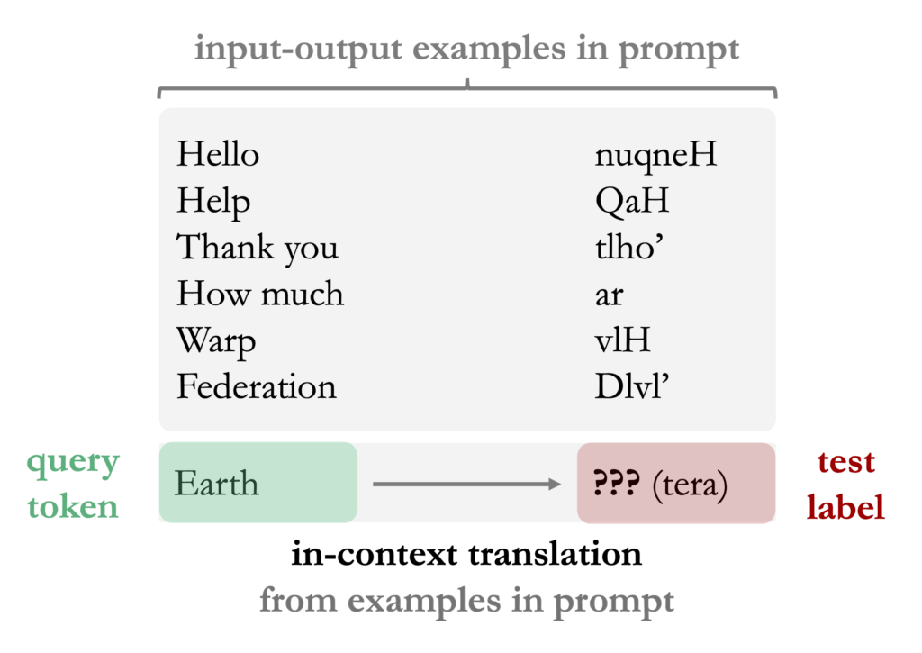
Figure 1: Example of English-to-Klingon translation in-context. The model (pretrained on large amounts of text data, likely including English and Klingon) conditions on a few examples of English-to-Klingon pairs in order to perform the translation when prompted on a new query word (Earth).
Simultaneously, theoretical studies explore ICL using simpler architectures, such as linear attention or multilayer perceptrons, with mathematically well-defined tasks like regression, Markov chain inference, or dynamical system prediction. Here we will focus on in-context regression: a model is pretrained to predict outputs $f(x_{\ell+1})$ from a context of input-output pairs $(x_1, f(x_1)), \dots, (x_\ell, f(x_\ell))$ and a query input $x_{\ell+1}$. The model is exposed to a variety of tasks, i.e. different $x \to f(x)$ relationships, during pretraining, and is then evaluated on its ability to generalize to new relationships from the same family of functions. In this way, the model has learned to learn new functions from data purely via context, without any new parameter updates after pretraining.
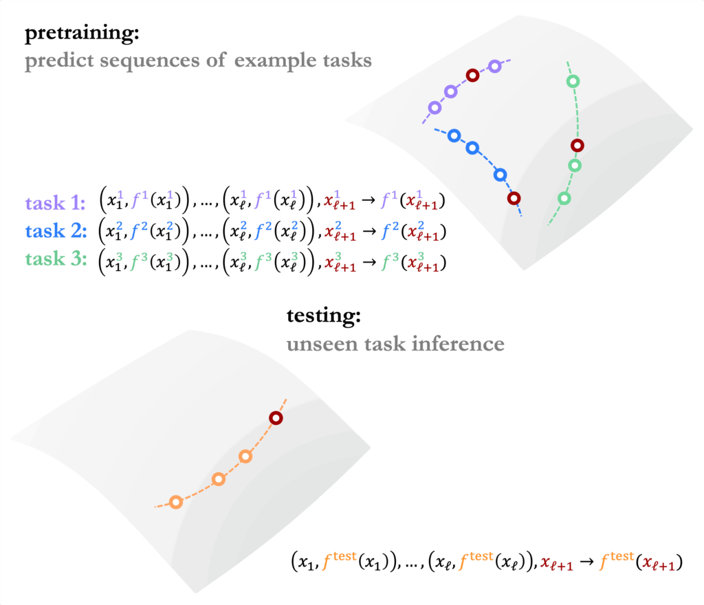
Figure 2: Illustration of an in-context regression setup. The model is pretrained on sequences of $(x,y)$ sample pairs for different tasks, and is then tested on a new task from the same family. Correctly predicting $f^\text{test}(x_{\ell+1})$ from the given sequence requires implicitly learning something about $f^\text{test}$.
Despite these differences, both the experimental and theoretical perspectives of ICL share the same key principle: pretraining exposes the model to a distribution over both tokens and tasks, and in-context learning emerges as the model’s ability to generalize to new tasks by conditioning on examples seen in input to perform this new task implicitly.
Key motivating questions
While in-context learning has been widely observed in large models pretrained on broad data distributions, the precise conditions causing this ability to emerge are not fully understood. What properties of the pretraining data, such as its size, diversity, structure, or task distribution, is necessary for ICL to emerge? How does the model’s architecture affect ICL performance? What is the role of the context length of sequences the model was pretrained to predict on? How many examples should be given in-context? How do the tasks seen during training affect what the model can learn in-context?
To progress in answering these questions, we study in-context learning of linear regression tasks using a linear attention model, in recent work with Yue M. Lu, Jacob Zavatone-Veth, Anindita Maiti, and Cengiz Pehlevan. By computing the asymptotic performance of ICL by this architecture in high dimensions, we are able to characterize how and when our model can generalize to new tasks, and give a precise description of what properties of pretraining data are necessary for ICL to emerge.
Building an analytically-solvable model
The structure of our data will follow what is illustrated in Figure 2, i.e. we will be studying in-context regression. We will specifically study linear regression, so we will be considering input sequences $$(x_1,y_1), (x_2,y_2), \cdots, (x_\ell, y_\ell), x_{\ell+1}$$ where $x \in \mathbb{R}^d$ and $y$ are related by a linear mapping $$y_i = \langle x_i, w\rangle + \varepsilon_i\,.$$ Here $\varepsilon_i$ is label noise and $w \in \mathbb{R}^d$ is called a task vector. The sequence length $\ell$ here is called context length.
We will chose an embedding of this input sequence that works well with the linear attention architecture we want to use later, $$Z = \begin{bmatrix} x_1 & x_2 & \cdots & x_\ell & x_{\ell+1} \\ y_1 & y_2 & \cdots & y_\ell & 0 \end{bmatrix}$$ where the 0 is a placeholder for the $y_{\ell+1}$ value that ultimately we will pretrain the model to predict. This $Z$ will be inputted to a simple linear attention module $$A(Z) := Z + \frac{1}{\ell}(VZ)(Z^\top M Z)$$ for value and attention matrices $V,M \in \mathbb{R}^{(d+1)\times (d+1)}.$
The output $A(Z)$ of this architecture is a matrix, but we only care about the value corresponding to $y_{\ell+1}$, i.e. the bottom-righthand value. Thus our predictor will be $$\hat{y}_{\ell+1} = A(Z)_{d+1, \ell+1}.$$
Expand the value and attention matrices into components $$V = \begin{bmatrix}V_{11} & v_{12} \\ v_{12}^\top & v_{22}\end{bmatrix}\,, \qquad M = \begin{bmatrix}M_{11} & m_{12} \\ m_{12}^\top & m_{22}\end{bmatrix}.$$ In our paper we consider a more general setting, but for the purposes of illustration here, the predictor $\hat{y}_{\ell+1}$ can be well-approximated by $$\hat{y}_{\ell+1} \approx \langle \Gamma, H_Z \rangle$$ for feature matrix $$H_Z : = \frac{1}{\ell}x_{\ell+1}\sum_{i=1}^\ell y_i x_i^\top \in \mathbb{R}^{d\times d}$$ and parameter matrix $$\Gamma := v_{22}M_{11} \in \mathbb{R}^{d\times d}.$$ As seen by this simplified form of the parameters, not all of the value and attention components are necessary for accurate prediction of $y_{\ell+1}$.
Learning algorithm intuition
Note that this immediately gives us some insight into how single-layer linear attention is solving the problem. Using that $y_i \approx w^\top x_i$ we see that $$\hat{y}_{\ell+1} \approx \langle \Gamma, x_{\ell+1}w^\top \hat{\Sigma}_x\rangle$$ for empirical token covariance $\hat{\Sigma}_x = \frac{1}{\ell}\sum_{i=1}^\ell x_ix_i^\top$. Thus, if our parameter matrix learns the inverse of the token covariance, i.e. $\Gamma = \Sigma_x^{-1}$, then we’d have $$\hat{y}_{\ell+1} \approx w^\top x_{\ell+1}$$ which is precisely the required answer.
In actuality, $\Gamma$ will be set by minimising the MSE loss between our predicted label $\hat{y}_{\ell+1}(Z) = \langle \Gamma, H_Z\rangle$ and the true label $y_{\ell+1}$.
Full pretraining dataset
So far we’ve considered a single $Z \to y_{\ell+1}$ pretraining point, defined by a single task vector $w$. For in-context learning to emerge, the model will need to see more than one task, and thus our pretraining set should contain $Z,y$ defined by different task vectors.
We define a pretraining set of sample size $n$ by $$(Z^1,y_{\ell+1}^1), (Z^2,y_{\ell+1}^2), \cdots, (Z^n,y_{\ell+1}^n).$$ For each different sample, the task vector $w$ that defines the $x\to y$ linear relationship can change. In particular, we let there be $k$ unique tasks $$\{w_1,\cdots,w_k\}$$ during pretraining, and we call $k$ the task diversity. When chosing a task to define a given $(Z,y)$ pair, we choose from this set of $k$ tasks uniformly.
If the number of pretraining samples $n$ is smaller than $k$, this means that each $(Z,y)$ sample is more likely to be defined by a unique task vector $w$. However, if $n$ is larger than $k$, then some $(Z,y)$ samples certainly share a task vector, even though they don’t share tokens $x$. In this way, we have limited the number of unique tasks that the model sees during pretraining, which allows us to quantify how many tasks are necessary for ICL to emerge.
To summarize, we have introduced 4 key parameters:
- token/task dimension $d$
- context length $\ell$, i.e. the length of the $(x,y)$ sequences that define $Z$
- pretraining sample size $n$
- and pretraining task diversity $k$.
Explicitly, we sample everything i.i.d. from isotropic Gaussians, for each sample context $\mu = 1,…,n$, sequence element $i = 1,…,\ell+1$, and pretraining task $j = 1,…,k$.
$$\text{tokens } x_i^\mu \sim \mathcal{N}(0,I_d/d)$$
$$\text{noise } \varepsilon_i^\mu \sim \mathcal{N}(0,\rho)$$
$$\text{task } w_j \sim \mathcal{N}(0,I_d)$$
Because we’re working with a simplified model, optimizing the regularized MSE loss between $\hat{y}_{\ell+1}$ and $y_{\ell+1}$ gives an analytic formula for optimal parameters $\text{vec}\left(\Gamma^*\right).$
Testing on new tasks
Now that we have our ‘pretrained’ model explicitly in terms of $\Gamma^*$, we want to actually test it on a new task $w^\text{new}$ (similar to Figure 2). For this, we can sample a fresh sequence $$(x_1,y_1), (x_2,y_2), \cdots, (x_\ell, y_\ell), x_{\ell+1}$$ for $$y_i = \langle x_i, w^\text{new} \rangle + \varepsilon_i$$ and compute the error between the predictor $\langle \Gamma^*, H_{Z^\text{new}}\rangle$ and the true label $\langle x_{\ell+1}, w^\text{new} \rangle$. This will be how we determine in-context performance: doing well on this test means the model has learned, from pretraining, to be able to infer arbitrary $w^\text{new}$ from samples.
We can then average over the Gaussian randomness in the tokens, noise, and tasks, to find a formula for $\Gamma^*$ as well as take an average over these test tasks to find the trained model’s average ICL performance. We derive a formula for this test error, which we call $e_\text{ICL}(\Gamma^*)$.
Testing on the same pretraining tasks
It will be also helpful to understand how well $\Gamma^*$ does on the tasks that it’s already seen during pretraining. This is not a test of in-context learning, but rather will help us gauge how strongly the model was influenced by its pretraining tasks; we call this in-distribution generalization. For this test, sample $w^\text{seen before}$ uniformly from the same set of tasks as pretraining, $\{w_1,…,w_k\}$. Generate the sequence $Z$ and label $y_{\ell+1}$ by sampling new tokens $x_i$ and noise $\varepsilon_i$, and compute the error between predictor $\langle \Gamma^*, H_{Z^\text{seen before}}\rangle$ and the true label $\langle x_{\ell+1}, w^\text{seen before} \rangle$. In this way, we are testing the model’s ability to perform a regression (given different samples) of a task that it’s seen before.
We derive a formula for this test error, which we call $e_\text{IDG}(\Gamma^*)$.
These formulas, $e_\text{ICL}(\Gamma^*)$ and $e_\text{IDG}(\Gamma^*)$, lead to various key insights, two of which we highlight here.
Parameter scalings
Recall the four key parameters of this model: $d$, $\ell$, $n$, $k$. It is not obvious a-priori how these should scale with each other for non-trivial ICL phenomena to emerge in this model. We identify these scaling relationships, by defining three asymptotic parameters that stay constant as token dimension $d$ gets larger:
$$\alpha \equiv \frac{\ell}{d}, \qquad \kappa \equiv \frac{k}{d}, \qquad \tau \equiv \frac{n}{d^2}.$$ These parameters can be interpreted inuitively as follows.
- Context length $\ell$ should scale linearly with token dimension $d$. This is familiar from standard linear regression, and intuitively we can think about this from the perspective of how many samples $x_1,…,x_\ell$ it would take to accurately estimate the statistical structure of the tokens. As we’ve seen previously from the intuitive description of this model, accurately estimating the sample covariance $\hat{\Sigma}_x$ is key for good ICL performance.
- Task diversity $k$ should scale linearly with token dimension $d$. Here a similar intuition applies, as we need to correctly estimate the statistics of the tasks we see during pretraining to be able to have a good estimate of the full task manifold.
- Finally, number of pretraining samples $n$ should scale quadratically with token dimension $d$. This can be understood by considering the view of the linear attention module itself: there are $d^2$ free parameters (i.e. $\Gamma$) and $n$ data points $Z \to y_{\ell+1}$ that the model sees during pretraining.
Our work identifies interesting phenomena in each of these scaling parameters. In particular, there is a double descent phenomena that occurs in $\tau$. For the purposes of this blog, we will focus on the task diversity parameter $\kappa$ and how our results show clearly the effect of this parameter on the emergence of ICL.
Task generalization vs. pretraining memorization
Here we focus on the effect of task diversity $k$. We will work in terms of the scaling parameter $$\kappa = \frac{k}{d}.$$ Intuitively, one may think that seeing more tasks (larger $k$ relative to $d$) should make the model better at in-context learning. Conversely, seeing fewer tasks should make the model worse at in-context learning.
We wish to precisely answer if and when a model is actually learning in-context, i.e., genuinely solving a new regression problem by adapting to the specific structure of the task, rather than relying solely on memorized training task vectors. To do this, we will define a measure of task generalisation $$g_\text{task} = e_\text{ICL} – e_\text{IDG}.$$ What does this mean, and why does it represent task generalization?
- First of all, $g_\text{task} \geq 0$, for the simple reason that generalizing to learn $w^\text{new}$ will always be harder than learning $w^\text{seen before}.$
- Suppose $g_\text{task} = 0$. Then $e_\text{ICL} = e_\text{IDG}$, and so the model performs exactly the same when tested on $w^\text{new}$ vs when tested on $w^\text{seen before}$. The fact that $w^\text{seen before}$ is part of the pretraining task set has no effect on the model’s performance. In this way, the model has achieved true task-generalization as it’s not relying at all on any pretraining-specific knowledge.
- On the other hand, if $g_\text{task}>>0$, then the model is performing much better on the IDG test than the ICL test: the model has learned to perform regression well on tasks seen during pretraining, but cannot generalize to new tasks. Here the model is more likely to be memorizing pretraining tasks.
By studying $g_\text{task}$ and how it changes with the amount of pretraining tasks (measured with $\kappa$), we can understand how many unique tasks a model needs to be exposed to before it can generalize to any new task. For the linear transformer, using our formulas, we show that (in the limit of large pretraining size $n$ and large context length $\ell$) there’s a task-generalization phase transition! Explicitly, $$g_\text{task} \to \begin{cases} \left(1+\frac{\rho}{1+\rho}\right)(1-\kappa) & \kappa < 1 \\ 0 & \kappa > 1 \end{cases}\,.$$
This result shows that the linear attention mechanism is an extremely efficient task generalizer, evidenced by this sharp collapse to task-generalization as soon as $k = d$.
For comparison, Raventos et al introduce a ‘memorizer’ predictor, called dMMSE, that given a new context $(x_1,y_1),(x_2,y_2),…,(x_\ell,y_\ell)$ picks a task from the training set $\{w_1,…,w_k\}$ to use as its predictor. Note that this dMMSE predictor, by construction, will perform optimally on the IDG test, when the task defining the new context actually _is_ a training vector. However, it will not be optimal on the ICL test.
We show that the $g_\text{task}$ measure for the dMMSE predictor decays in $\kappa$ exponentially slowly, while the linear attention model, as seen above, has a sharp transition to $g_\text{task}$.
Even better, this sharp transition persists in nonlinear attention-based models on the same linear regression setup, showing transferable insights beyond our toy setup. Our results here indicate that the attention mechanism (either linear or nonlinear) learns a much better implicit algorithm for inferring $w$ from samples than a pure memorizer.

Figure 3: Plots of $g_\text{task}$ against $\kappa$; squares show $g_\text{task}$ for the dMMSE predictor, while circles show values for (A.) the linear attention theoretical setup and (B.) a transformer with softmax attention and MLP layers. Both exhibit a much much faster transition to task generalization than the dMMSE ‘memorization’ predictor. Note $\alpha = \ell/d$ is the context length scaling parameter.
Concluding thoughts
Our study shows that simple models like linear attention can exhibit rich in-context learning behavior. By identifying the precise relationships between token dimension, context length, task diversity, and sample size, we provide a precise formulas for ICL performance in a toy model, which allow us to better understand how it works. In particular, our proposed task generalization measure reveals that both our toy model and more realistic architectures can generalize to new tasks in-context far more effectively than a brute-force memorizer.
There is much more to explore within this framework. Our analysis here is limited to isotropic task distributions at both pretraining and test time. This restricts our ability to model how nontrivial task structure at pretraining shapes the model’s inductive bias and affects test-time generalization. Future work will explore how anisotropic task distributions and varying test-time context lengths affect ICL performance. These directions will deepen our understanding of how model architecture and data structure jointly shape the emergence of in-context learning.
Note: Various formulas and expressions have been shortened / simplified from their more general form provided in the article, for simplicity and intuition.