Loss-to-Loss Prediction

Scaling laws – which reliably predict the performance of large language models (LLMs) as a function of their size and the amount of data they have been trained on – have been the primary driver behind building today’s most capable AI models, such as Claude and GPT. While these laws help us understand how models improve with more compute and data, they’ve historically been limited to studying models trained on a fixed data distribution (for example, a broad collection of internet text).

Little is known about how model performance changes when we start changing the data distribution – for example, how does the performance of a model that was trained on both English and code compare with one only trained on code?  This is an important question for several reasons: (1) Training language models with hundreds of billions of parameters is extremely expensive, often costing millions of dollars per training run, so understanding how their performance scales as the training data is changed can lead to substantial cost savings and better capabilities. (2) We need reliable ways to measure and predict model performance across different types of data, helping us understand what our models are actually learning.  For example, how much of a model’s ability to write code transfers to its ability to write English, if at all? (3) From a purely curiosity-driven perspective, we would like to understand how different types of training data interact with the scale of compute, which in turn may produce insights about how to train more capable models.

Our approach

In a new preprint, we (David Brandfonbrener, Nikhil Anand, Nikhil Vyas, Eran Malach, Sham Kakade) propose a methodology to translate scaling laws obtained from one data distribution to another.  We then apply our method to:

1. Predict how a model trained on one dataset does when trained on a different dataset (these datasets can be very different; for example, some are all code while others contain no code);
2. Predict how well a model does on a held-out test set from its performance on training data;
3. Understand how the performance on a held-out test dataset changes as we start changing the training data.

The core finding of our work is that model performance, as measured through loss, follows predictable patterns when changing datasets and can be fit with a simple shifted power law. These trends hold even when comparing very different types of data, as long as we properly account for the compute used in training, and extrapolate well to 20x the compute used to generate the fits.

Review of scaling laws

Before diving into our results, let’s review how scaling laws work.  Scaling laws are empirically observed relationships that predict model performance (typically measured through the cross-entropy loss L), as a function of compute i.e. the number of model parameters N and the size of the training dataset D (in tokens).  The recent surge in building ever-larger language models was, in part, due to the work of Kaplan et al., who noticed that model performance scaled in a predictable way with N and D, spanning several orders of magnitude.  In particular, they found that there is a simple power law that relates the loss on a held-out validation set and N and D:

$$ L(N, D) = \left(\left(\frac{A}{N}\right)^{\alpha / \beta} + \frac{B}{D}\right)^{\beta} $$

where A, B, , are numbers fit from data. In Hoffman et al., this work was extended and refined to determine the scaling to obtain “compute-optimal” models. In that work, the scaling fit used broke apart N and D and included an entropy term (essentially the best possible performance achievable on that dataset):

$$ L(N, D) = E + \frac{A}{N^\alpha} + \frac{B}{D^\beta} $$

In our work we opted for a functional form that blends both of these forms:

$$ L(N, D) = E + \left(\left(\frac{A}{N}\right)^{\alpha / \beta} + \frac{B}{D}\right)^{\beta} $$

that permits a simple description of how loss translates between datasets (though we do not necessarily rule out other parametrizations).  However, regardless of the exact functional form used, the key point about scaling laws is that they offer a precise way to quantify model performance as a function of compute spent and are the starting point of our analysis.

Translating scaling laws: train-to-train

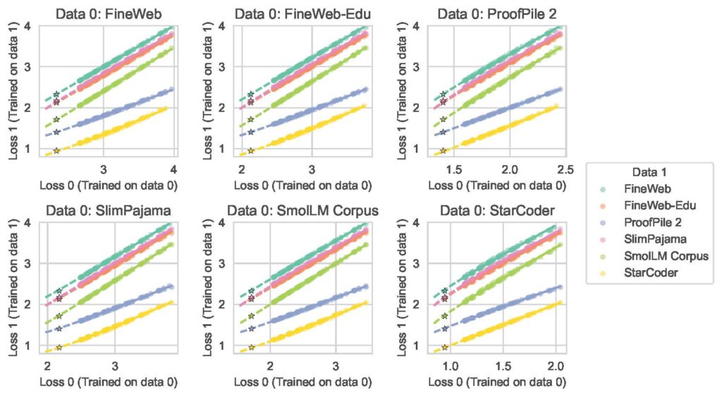
Our first key finding is that there exists a simple mathematical relationship between the training losses of models trained on different datasets when the models are paired up by compute.  Specifically, when we compare two models with the same number of parameters N trained on the same number of tokens D but on different datasets, their losses (L₀ and L₁) are related by a shifted power law:

$$ L_1 = K(L_0 – E_0)^{\kappa} + E_1 $$

Here, K and κ are parameters we fit from data, while E₀ and E₁ represent the irreducible entropy extracted individually from each distribution (they are not free parameters in the above fit). In other words, given two training distributions with an equal amount of compute to spend on training on data drawn from those distributions, we find that there is a simple power law that relates the losses on those datasets.  This relationship holds remarkably well across very different datasets  – from pure code to pure English text.  It is worth emphasizing that the above equation only has two free parameters to fit all of the data points – K and κ– yet it reliably holds for the entire experimental range of models we used to draw the fit, and extrapolates accurately to models 20 times larger than those used to fit the relationship.

In our experiments depicted in Fig. 2, we systematically varied model sizes from 20M to 1.7B parameters, with compute budgets ranging from 2e17 to 4.84e19 FLOPs. We tested this relationship across six diverse datasets: FineWeb, FineWeb-edu, Proof Pile 2, SlimPajama, SmolLM Corpus, and StarCoder.

We find that κ typically ranges from 0.88 to 1.13, with the most extreme differences occurring between StarCoder and SlimPajama.  K shows greater variation, reaching values from 0.55 to 1.72 between SmolLM Corpus and ProofPile.  We note that these variations aren’t random – they reveal fundamental differences in how efficiently different datasets can be learned; for example, directly tells us how the overall loss scaling exponent in our scaling equation translates between datasets.

Translating scaling laws: train-to-test

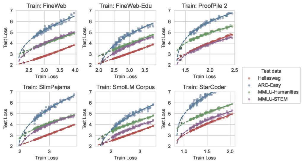
After establishing relationships between training losses, we investigated how training performance relates to test performance across different distributions. We found a similar shifted power law relationship:

$$ L_\text{test} = K(L_\text{train} – E_\text{train})^\kappa + E_{\text{test}|\text{train}} $$

where E_test|train represents the irreducible loss when evaluating on the test distribution for a model trained on the training distribution.  In practice, to estimate this quantity, we fit a scaling law on the test loss for all of the models trained on the training distribution, and extract the entropy term.  This relationship reveals, for example, when transferring from natural language datasets (like FineWeb) to code datasets (like StarCoder), we observe diminishing returns – the curves are convex (κ > 1), indicating that improvements in training loss yield progressively smaller gains in test performance. This suggests that even as models become extremely good at processing natural language, their ability to handle code doesn’t always improve proportionally.

Conversely, for many downstream tasks like ARC-Easy (a question-answering dataset), we see concave relationships (κ < 1), indicating increasing returns – improvements in training loss yield progressively larger gains in test performance. This pattern suggests that these capabilities may reside in the “tail” of the training distribution, only becoming accessible as models achieve lower training losses, further emphasizing the importance of data selection for downstream tasks.

Translating scaling laws: test-to-test

Finally, we can combine the above insights to understand how test performance compares across models trained on different datasets.  For example, how does a model perform on a question-answer test dataset when trained on code versus on synthetic data?  This involves defining three distributions: P₀ (initial training data), P₁ (new training data), and P_test (test distribution). Again, we find shifted power law relationships when comparing models paired by compute:

$$ L_\text{test}(f_1) = K(L_\text{test}(f_0) – E_{\text{test}|0})^\kappa + E_{\text{test}|1} $$

The content of the above equation is that the loss on the test dataset (left hand side), as determined using a model trained on P₁, can be related to the same test loss as determined through a model trained on P₀, through another shifted power-law. These relationships, while noisier than train-to-train predictions, reveal that asymptotic transfer performance on test sets can be substantially worse than performance achieved by training directly on that domain – even for seemingly similar data distributions like SlimPajama and SmolLM!  They are also typically predictive and extrapolate to 20x the FLOP budget of the points used to fit the curves, but tend to be noisier for some datasets.

Application: translating a scaling law

We can apply our translation methodology to a scenario that a practitioner may encounter: suppose you have already trained models extensively on one dataset and want to predict performance on a new dataset.  One option is to just train a few models in isolation on the new dataset and fit a scaling curve and then extrapolate performance.  But this wouldn’t be leveraging any information about the models we’ve already trained on the other dataset!  By incorporating this extra information that we already have, our method can provide remarkably accurate predictions with minimal additional computation.  The key point is that any given loss isn’t just a number that exists in a vacuum, but rather losses relate to each other in a rigid way as predicted by our transfer equations.  In our experiments, using just 8 models trained on a new dataset combined with our loss-to-loss prediction methodology yielded scaling law predictions nearly as accurate (R² within 0.001) as traditional methods requiring 88 models.

This is illustrated in Fig. 5, where 8 models trained on the target dataset (e.g., ProofPile-2) are enough to obtain a scaling law when combined with models trained on an existing dataset (FineWeb-Edu). 

Looking forward

While our work provides fundamental insights into how model performance translates across datasets, several questions remain:

• How can these relationships inform optimal dataset mixing strategies?
• What drives the surprisingly strong connections between seemingly unrelated domains?
• How do these relationships change with different model architectures?

For those interested in exploring further, we’ve released our code, notebooks, and trained models through the Kempner Institute’s GitHub repositories.