Interpreting the Linear Structure of Vision-Language Model Embedding Spaces

Vision-language models (VLMs) project images and text into a shared embedding space, enabling a wide range of powerful multimodal capabilities. But how is this space structured internally? In our work, we investigate this question through the lens of sparse dictionary learning, training sparse autoencoders (SAEs) on the embedding spaces of four prominent VLMs: CLIP, SigLIP, SigLIP2, and AIMv2, and analyzing the dictionary directions found in the embedding spaces.

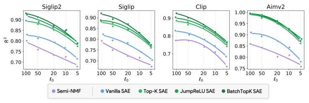
We find that, compared to other methods of linear feature learning, SAEs are better at reconstructing the real embeddings (high $R^2$), while also being able to retain the most sparsity (low $\ell_0$).

Retraining SAEs with different seeds and different image:text data mixtures leads to two findings: the rare, specific concepts captured by the SAEs are liable to change drastically, but the key commonly-activating concepts extracted by SAEs are remarkably stable across runs.

Interestingly, while most concepts activate almost exclusively for one modality, we find they are not simply encoding modality. Many concepts are almost orthogonal – but not entirely orthogonal – to the subspace that defines modality, meaning that they are encoding cross-modal concepts. To quantify this bridging behavior between modalities, we introduce the Bridge Score, a metric that identifies concept pairs which are both co-activated across aligned image-text inputs and geometrically aligned in the shared space. This reveals how single-modality concepts collaborate to support cross-modal integration.

We release interactive demos of the concepts and metrics for all models, allowing researchers to explore the organization of concept spaces.

Background: Sparse Autoencoders for Dictionary Learning

We begin by framing our approach as a dictionary learning problem. Given a large matrix of embeddings $A \in \mathbb{R}^{n \times d}$ from a VLM — produced by passing text and image inputs through the model — we aim to approximate each embedding as a sparse linear combination of a learned dictionary $D \in \mathbb{R}^{c \times d}$ with code matrix $Z \in \mathbb{R}^{n \times c}$: $$ (Z^\star, D^\star) = \arg \min_{Z, D} \|A – ZD\|_F^2 \quad \text{s.t.} \quad \|Z_i\|_0 \leq k \quad \forall i $$ Specifically, we implement this with BatchTopK Sparse Autoencoders, where the encoder applies a top-$k$ operator $\Pi_k \{\cdot\}$ to enforce sparsity: $$ Z = \Pi_k \{ AW + b \}, \quad \text{with } \Pi_k(x)_i = \begin{cases} x_i & \text{if } i \in \text{Top-}k(x) \\ 0 & \text{otherwise} \end{cases} $$ Each row of $Z$ selects a small number of concepts from $D$ that best reconstruct the original embedding. This discrete selection enforces interpretability and compresses the space into meaningful directions.

Evaluating the Learned SAE Concepts

To understand and evaluate the dictionaries and sparse codes produced by our SAEs, we introduce four key metrics:

Reconstruction Error

We measure how well the SAE approximates the input activations. This is the core loss used in training: $$ \text{Error} = \|A – ZD\|_F^2 $$ Or normalized as an $R^2$ score: $$ R^2 = 1 – \frac{\|A – ZD\|_F^2}{\|A – \bar{A}\|_F^2} $$ where $\bar{A}$ is the mean of the dataset.

Energy

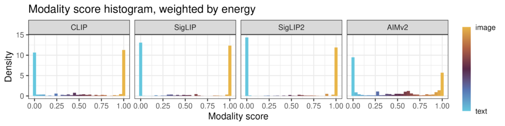
Energy quantifies how strongly and frequently a concept is used. For concept $i$, we define: $$ \text{Energy}_i = \mathbb{E}_{z \sim \mathcal{D}} [z_i] $$ In practice, we average $z_i$ over all activations in the dataset. Concepts with high energy are critical for reconstruction and interpretation.

Stability

We want our learned dictionaries to be consistent across retrainings. For two dictionaries $D, D’ \in \mathbb{R}^{c \times d}$, we compute stability by finding the best permutation $P$ of the rows that maximizes cosine similarity: $$ \text{Stability}(D, D’) = \max_{P \in \mathcal{P}(c)} \; \frac{1}{c} \mathrm{Tr}(D^\top P D’) $$ We use the Hungarian algorithm to solve for the optimal $P$. Stability is high when concepts are similar across runs.

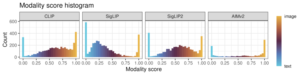
Modality Score

This measures whether a concept is used mostly by image embeddings or text embeddings. Given distributions $\iota$ and $\tau$ over image and text activations: $$ \text{ModalityScore}_i = \frac{\mathbb{E}_{z \sim \iota}[z_i]}{\mathbb{E}_{z \sim \iota}[z_i] + \mathbb{E}_{z \sim \tau}[z_i]} $$ A score close to 1 means the concept is image-specific, while a score close to 0 implies it is text-specific.

Bridge Score

To quantify cross-modal alignment, we define a bridge matrix $B \in \mathbb{R}^{c \times c}$. For paired image-text embeddings $(z_\iota, z_\tau) \sim \gamma$, the bridge score combines co-activation and directional alignment: $$ B = \mathbb{E}_{(z_\iota, z_\tau)} \left[ z_\iota^\top z_\tau \right] \odot \left( D D^\top \right) $$ Here $\odot$ is the Hadamard product. A large value of $B_{i,j}$ indicates that concept $i$ (from image) and $j$ (from text) are both (1) co-activated and (2) geometrically aligned—forming a semantic bridge.

A Consistent High-Energy Core

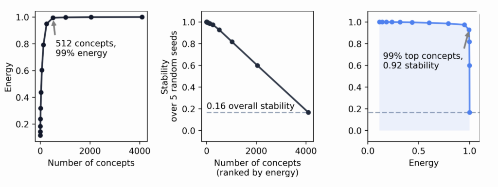
If we run the same SAE with two different seeds, will the two runs recover similar concepts? We find that, though there is actually considerable variance between runs, the concepts that are most often activated are consistent across runs. These high energy concepts form a stable basis for interpreting the model. When comparing dictionaries across different seeds, the overall stability is low: $$ \text{Stability}_{\text{all}} \approx 0.16 $$ But if we restrict to the top 512 most-used concepts, stability rises dramatically: $$ \text{Stability}_{\text{top-512}} \approx 0.92 $$

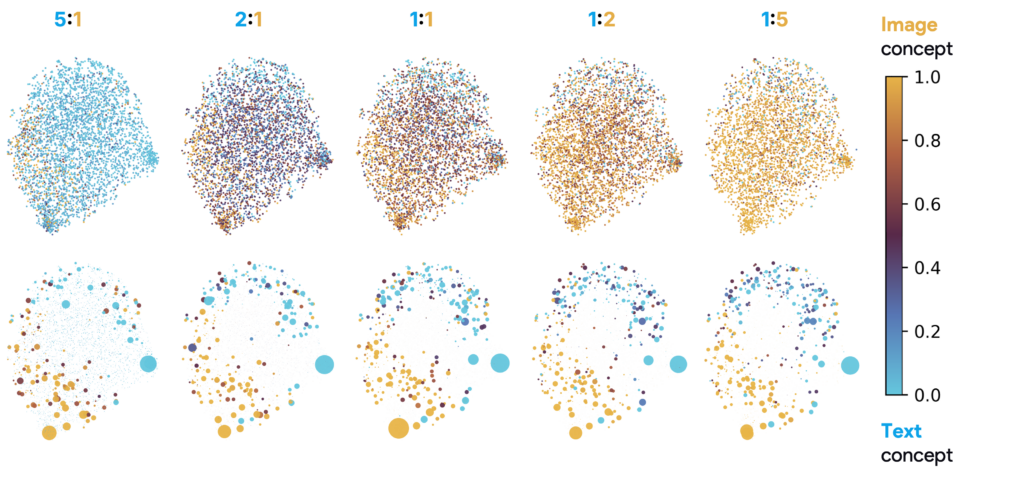
We find something similar when we train SAEs with different ratios of embeddings from text or images. The training data ratio influences what concepts are found overall (eg, more text embeddings mean that the SAE finds text-specific concepts), but the highest-energy concepts remain constant. We demonstrate this in a UMAP visualization of the concepts in CLiP, where on the bottom row we have weighted each point by its energy:

Key finding: the apparent instability of SAEs is due to rare, low-energy concepts. Once we condition on energy, the core concepts emerge as stable and semantically meaningful.

Single-modality Usage, Cross-Modal Structure

When we analyze SAE concepts by their modality scores (how much each concept activates for text vs for image inputs), we find that nearly all high-energy concepts are single-modality in usage, activating primarily on either images or text.

However, we know that the latent spaces of VLMs have some type of cross-modal structure, as the vision-language training objectives specifically achieve that. Using the bridge matrix $B$, we can see that concepts of different modalities activate for semantically linked image-caption pairs, and that these same concepts often have high cosine similarities. This means that, despite being functionally unimodal, concepts can form semantically meaningful cross-modal bridges through high co-activation and directional alignment.

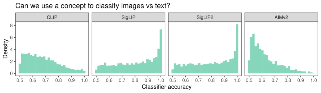
Another way of analyzing whether concepts encode cross-modal information is to check how aligned they are with the subspace that encodes modality. We do this by checking if SAE concept directions can act as good classifiers for classifying modality. If there is a linear subspace that largely defines modality in the model space, concepts can be aligned with the subspace (in which case projecting data points onto the concept direction can give us an accuracy of 100% separability) or orthogonal to the subspace, lying on a modality-agnostic subspace (in which case the projection will give us at-chance accuracy).

We find that many concept vectors are nearly orthogonal to the modality subspace — i.e., they don’t linearly separate text from images. That means that they lie almost on (but not perfectly on) a modality-agnostic subspace.

Geometry vs. Functional Use: The SAE Projection Effect

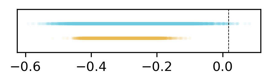
So, how is it that concepts only activate for a single modality, but aren’t geometrically aligned with the modality direction, and in fact create cross-modal semantic bridges between modalities through their directional alignment? We posit that this is due to the SAE projection step, where concepts only fire if they pass a sparsity operator. $$ Z = \Pi_k \{ AW + b \} \quad \text{selects top } k \text{ entries per input} $$ Even slight asymmetries can yield sharp modality skew in concept usage, even if the underlying direction is largely cross-modal. For example, if below (Figure 7) we plot the dot product of text (blue) and image (orange) embeddings with a single concept, we can see that the concept does not separate the two modalities very well. However, due to the top-k step, the concept only activates for embeddings above the dotted line — meaning that it only ever activates for text concepts, despite being almost modality-agnostic in its direction.

Visualizing the Concept Space: VLM-Explore

To explore these dictionaries, we developed VLM-Explore, an interactive UMAP-based tool that displays:

• Each concept, colored by modality score and sized by energy
• Top-activating samples (image or text) for each concept
• High-bridge-score connections between concept pairs

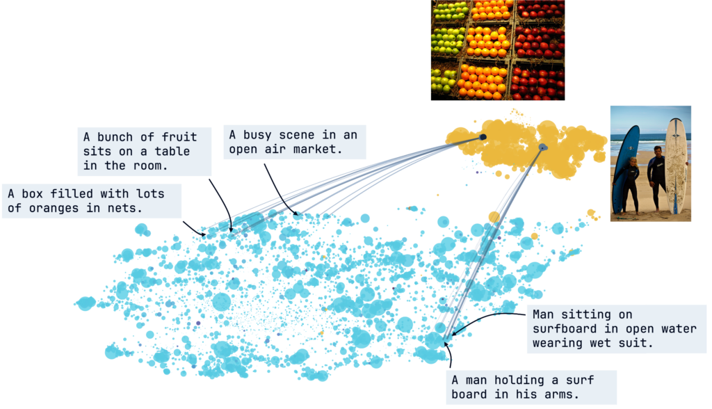
This tool allows researchers to visualize how concepts link across modalities and examine many-to-many alignments—like “red bus” or “wooden texture”—that support the model’s semantic representations.

Conclusion

Our work uncovers a sparse linear structure inside vision-language embedding spaces:

• A small, high-energy subset of concepts drives almost all reconstruction
• These concepts are stable across seeds and robust to data variation
• Despite strong single-modality usage, cross-modal alignment emerges via co-activation and geometric bridges
• Many concepts are modality-neutral in direction but appear to be single-modality due to the SAE projection effect

These findings offer a new lens on how multimodal representations are composed—and suggest that sparse autoencoders can serve as reliable, interpretable tools for studying and improving vision-language models.