Characterization and Mitigation of Training Instabilities in Microscaling Formats

What precision—that is, how many significant digits—do we need to train large language models? For instance, must a number be stored as 3.14159, or is 3.14 sufficient? This seemingly simple question has in fact inspired a great deal of research over the past few years, as the answer carries many implications for the cost and feasibility of developing frontier AI models.

The landscape of precision

First, let’s understand the tradeoffs. Training large models is an expensive, compute-bound process.  If we reduce the precision of a computation, such as a typical matrix multiplication (matmul) that happens on a GPU, we theoretically increase the throughput and shorten the wall-clock time AKA dollars needed to train our model. Intuitively, this makes sense since multiplying 3.14 by 1.43 should be faster than multiplying 3.14159 by 9.51413. However, this speed-up can come at the cost of accuracy and the error from rounding numbers can accumulate over billions of operations and potentially harm model performance.

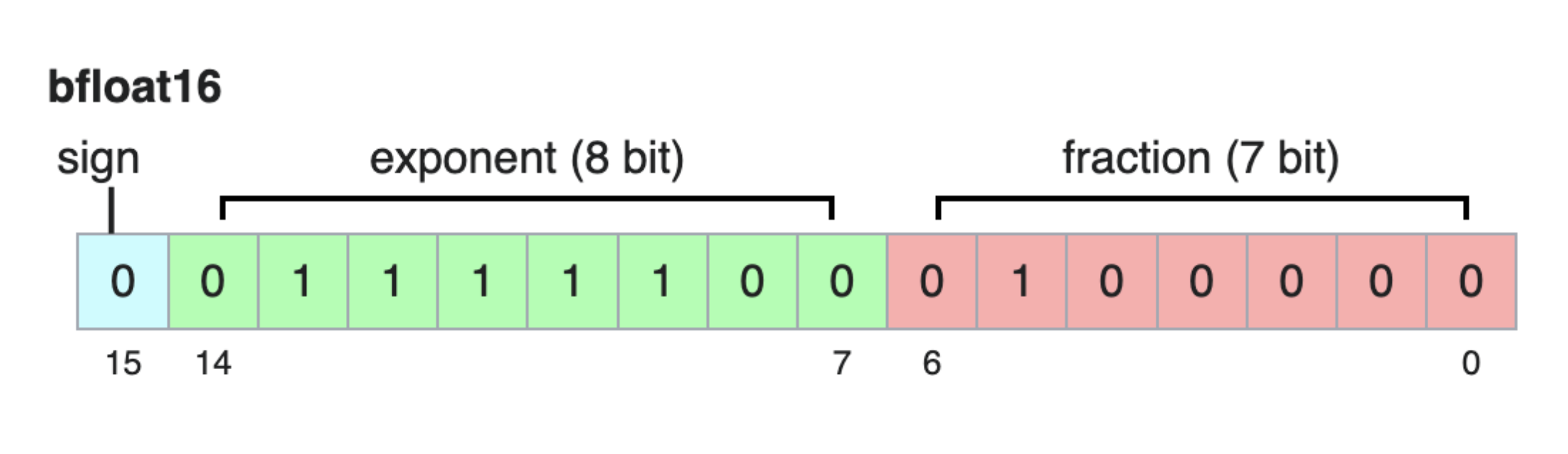
The last decade has seen a rapid, tightly-coupled evolution in hardware and software to navigate this tradeoff. The industry standard was once 32-bit single-precision floating-point (FP32). Then, NVIDIA’s Volta architecture (2017) introduced Tensor Cores that accelerated half-precision (FP16) matmul. A year later, Google Brain designed the bfloat16 format for its TPUs, which preserved the wide dynamic range of FP32 while using only 16 bits. This was followed by formats like NVIDIA’s TF32 and, more recently, two 8-bit floating-point (FP8) formats accelerated by the Hopper architecture and, more recently, even 4-bit formats on Blackwell.

Typical pretraining setups involve using high precision formats, such as bfloat16 for arithmetic computations.  However, some production LLMs are seeing even pretraining happening in even lower precision, such as the upcoming Llama 4 model or Cohere’s Command A model, which are reported to be trained in FP8.  Then, there are post-training protocols such as quantization aware training (QAT) and post training quantization (PTQ) that aim to prepare the model for deployment in lower precision since inference FLOPs can easily be larger than the FLOPs used in model training.  Underlying all of this, however, is the critical need to understand exactly how low precision formats impact any process involving gradient-based updates.

Hardware manufacturers like NVIDIA are aware of these constraints, and frontier labs are pushing ever harder to make models bigger, train these models on more data, and release them at a faster cadence.  Amplifying the compute demand is the fact that models have to be trained, and retrained, as new data comes in and algorithms evolve.

To meet these compute demands and support lower-precision formats, one must contend with several technical problems, including the core challenge of a limited dynamic range: the span between the smallest and largest representable numbers. Naïve quantization can “clamp” large values or “zero out” small ones, both of which are detrimental to learning.

To address this, scaled quantization was developed. The idea is simple: for a group of values, a single scale factor is computed. Each value is divided by this factor to bring the entire group into an acceptable range before it’s converted to low precision. These scale factors are then used to restore the original magnitude after the computation is complete.

Upcoming hardware accelerators powered by NVIDIA’s Blackwell architecture will standardize this approach with built-in support for shared-scale Microscaling (MX) formats, like MXFP8 and MXFP6. By storing a scale factor for each small block of parameters (e.g., 32 values), these formats expand the effective dynamic range with minimal overhead, promising the efficiency of low-precision GEMM operations without the typical range limitations.

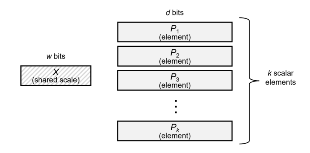
An illustration of how these formats work is shown in Figure 2 (at right).  The MX block quantization algorithm converts a high-precision vector into a low-precision representation by first computing the maximum absolute value within a block and using it to define a shared power-of-two scale factor. Each element is then divided by this scale and quantized to a low-precision format. This preserves dynamic range across the block while enabling efficient storage and computation. Of course, there are alternative methods, such as doing tilewise quantization rather than by block, but these formats provide a good baseline for how the new Blackwell formats go.

Training instabilities in lower precision

Our paper takes a close look at the viability of block-scaled formats such as MX formats for model training. In our work, we trained nearly a thousand language models spanning 2e17 – 5e19 FLOPs with different combinations of precision formats for both weights and activations. This includes the reduced precision in the backward pass.  For example, we might train with MX FP8 E4M3 for weights and MX FP8 E5M2 in the activations, where EXMY refers to the X  exponent and Y mantissa bits.

Surprisingly, we found that every combination of formats eventually led to training instabilities, especially when the larger models were trained for longer. The language models used in our experiments were based on the OLMo architecture, making them representative of models used in practice.

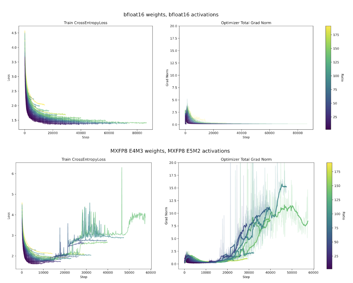
While low-precision formats are expected to be less stable, the failures observed here were pervasive and consistent. In nearly all the language models trained from scratch on FineWeb-Edu (a standard, relatively clean pretraining dataset), the gradient norm grew uncontrollably before the loss spiked. This suggested a deeper, systematic issue with how gradients were being biased during optimization.

A synthetic model to isolate the problem

Because so many variables are entangled in a billion parameter language model, it’s intractable to reason about its complex dynamics and isolate the effect of precision. To get a small-scale proxy for what was going on with the language model, we turned to a synthetic student-teacher model, in which the student neural network is a simple residual multi-layer perceptron (MLP), which captures the core computational patterns of a Transformer block (like residual connections and layer normalization) while avoiding the complexity of attention mechanisms.

This proxy model, despite its simplicity, exhibits the same training instabilities seen in the full-scale language models. Because the setting is carefully controlled, with identical initializations, data, and batch orders, any difference in behavior between a full-precision run and a low-precision run can be directly attributed to the numerical format.

This synthetic setup allows for fine-grained experiments that would be impossible or computationally prohibitive in a large-scale setting. By ablating different components like activation functions or layer normalization, and by sweeping across hyperparameters like the learning rate, it becomes possible to pinpoint exactly what triggers the catastrophic divergence.

We found that that there are two types of instabilities:

1. The first is “expected” and stems from stochastic optimization dynamics: for instance, aggressive learning rates can amplify small incorrect gradient updates, resulting in loss spikes and divergence.
2. The second, perhaps more interesting, mode is directly induced by low-precision arithmetic: even under stable hyperparameters, quantization introduces systematic gradient bias that accumulates and destabilizes training.  

Understanding low-precision dynamics

Where does the bias from the second case come from? In microscaling formats, the shared scale helps to keep most values within a representable range so it is difficult to understand how we can get overflow or underflow issues. Our experiments support the evidence for a subtle interaction between the properties of the low-precision format and the distribution of the values being quantized—particularly the affine weights in layer norm layers.

To understand this, let’s examine the specifics of the MXFP8 E4M3 format. It uses 8 bits, but not all represent distinct positive numbers. One bit is for the sign. Of the 127 positive patterns, one is reserved for the zero code and another (S 1111 111) is reserved for the NaN (Not a Number) symbol. This leaves 125 distinct positive values that can be represented.  The “sawtooth” plot below (Left) shows the relative percentage gap between successive representable numbers in this format. Notice two things:

1. Within each exponent range, the precision varies, with the relative gap shrinking from 12.5% down to 6.6%.
2. Once a scaled value exceeds the largest representable number (448), it gets clamped. This is the “overflow region” shown in gray.

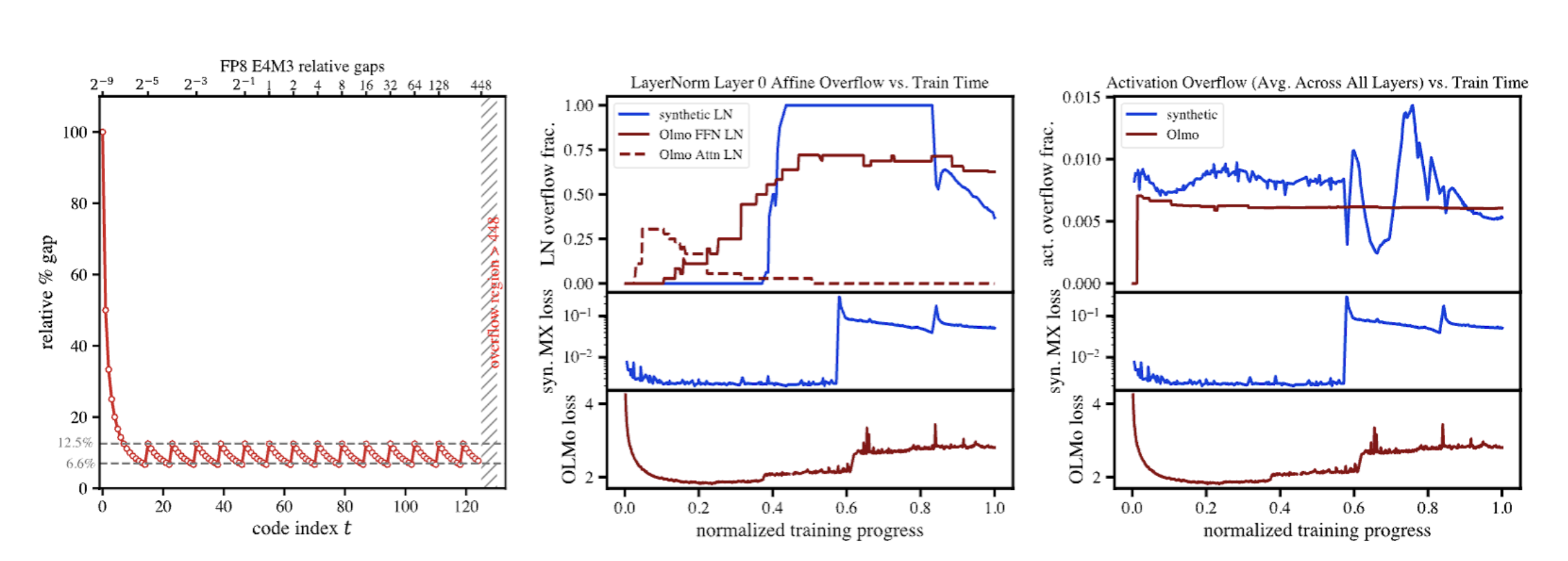
Due to the definition of the MX FP8 E4M3 format, a value gets clamped to this overflow region if its magnitude is greater than 87.5% of the absolute maximum value within its 32-element block in the MX FP8 E4M3 format.  Why is this the case?  The shared scale is chosen to be the closest power-of-2 to the absolute max within a block, minus the exponent of the largest representable value (in this particular format, 8).  If the values within a block lie close enough to each other and if the closest representable power of 2 is small enough, we can end up dividing an entire block by a small number like 2^-8 and, if they’re all within a narrow enough band, overflow into the grey region.  

Generically, we don’t expect this to be true, for example, if the values were distributed randomly according to a uniform distribution of sufficient width… it takes a specific kind of distribution for this to happen!  Interestingly, layer norm affine parameters follow exactly the kind of log-normal distribution to see this effect.  These parameters tend to be very tightly clustered around a value close to 1.0. When this happens, it’s very likely that all 32 weights in a block fall into the overflow region after shared scale division, quantized to the exact same number, and any variation between them is erased.

Mitigations

Once we’ve identified the cause of the instability, we can figure out how to fix it.  Our work explored several mitigation strategies, moving from general changes to the training recipe to targeted, last-minute interventions designed to prevent an impending instability.

Two general strategies were tested to see if they could improve stability from the start:

• Quantizing only the forward pass: This approach avoids introducing quantization noise into the gradient computations of the backward pass.
• Using higher-precision activations: Here, the model weights are kept in a low-precision MX format, but the activations (including the outputs of layer norm layers and computations involving the LN weights) are maintained in a higher-precision format like bfloat16.

Can you save a run that’s about to fail?

To dig deeper, we designed an experiment to see if an impending divergence could be averted with a last-minute intervention. We took a model configuration that we knew was stable in full precision but failed consistently in MXFP8 E4M3 around step 5,100. We then applied different fixes either well before the failure (at step 4,500) or right before the crash (at step 5,080) to see if we could save the run (seen in figure below).

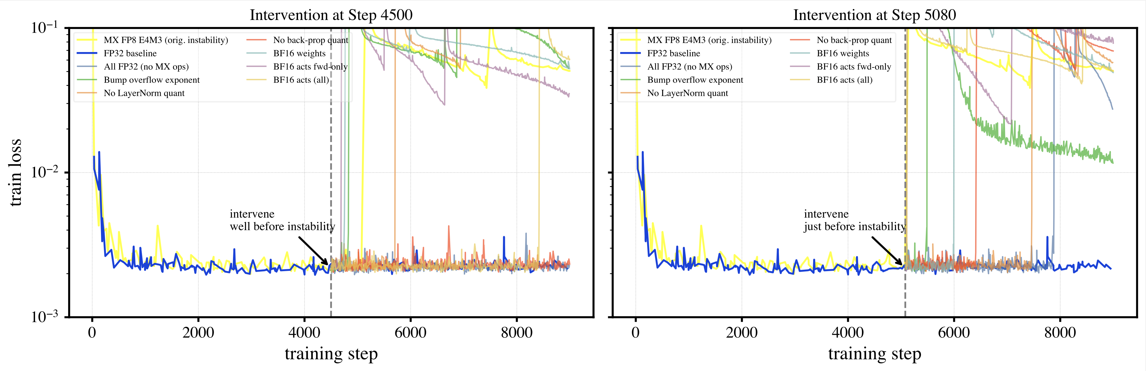
The results of these “in-situ” interventions were:

• Switching to Full Precision (FP32): We found that the most drastic fix—switching the entire model to high precision—worked, but only if applied early. An early switch at step 4,500 prevented the crash entirely, but applying it at step 5,080 only delayed the inevitable, suggesting the accumulated quantization error had already done irreparable damage.
• Targeting the Layer Norm: We observed that specifically exempting the layer norm affine weights from quantization significantly delayed instability at both early and late intervention points.
• A Simple Fix That Didn’t Work: We tested a simple idea to just “bump” the shared exponent by one to avoid the immediate overflow issue, but found it had no large effect on stability. This indicated to us that the problem is more complex than a simple off-by-one error in the scale, and that a more nuanced scheme might be needed.

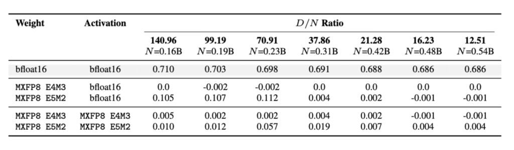
These fixes also worked on the full-scale language models. When applied back to the OLMo training runs, both strategies enabled stable training.  For example, training with MXFP8 E4M3 weights and bfloat16 activations achieved performance that was competitive with the full bfloat16 baseline across the model sizes we tested.  The results are shown in the table below.

Future directions

These experiments showed that while the instabilities from low-precision training can become irreversible, practical and effective strategies exist. We concluded that the most promising approaches involve protecting the activations and gradient calculations from quantization.

Looking ahead, future research can build on these insights in several key areas:

• Improving the Proxy Model: Extending the simple synthetic model to include more complex components like attention mechanisms and Mixture-of-Experts (MoE) could help predict instabilities in the next generation of state-of-the-art architectures.
• Developing a Clearer Theory: Building a formal mathematical theory around the observed stochastic noise could help us understand and predict precisely when and why training becomes unstable.

Designing Better Scaling Schemes: This research points to the need for new block-scaling algorithms that are smarter and more adaptive, especially for the skewed or tightly clustered data distributions that cause problems for current methods.