Anytime Pretraining: Horizon-Free Learning-Rate Schedules with Weight Averaging

Large language models are increasingly trained in continual or open-ended settings, where the total training horizon is not known in advance. Despite this, most existing pretraining recipes are not anytime: they rely on horizon-dependent learning-rate schedules and extensive tuning under a fixed compute budget. In this work, we provide a theoretical analysis demonstrating the existence of anytime learning schedules for overparameterized linear regression, and we highlight the central role of weight averaging—also known as model merging—in achieving the optimal convergence rates of stochastic gradient descent.

We show that these anytime schedules polynomially decay with time, with the decay rate determined by the source and capacity conditions of the problem. Empirically, we compare constant learning rates with weight averaging and $1/\sqrt{t}$-type schedules with weight averaging against well-tuned cosine schedules for language model pretraining. Across a wide range of training compute, the anytime schedules achieve comparable final loss to cosine decay, suggesting a practical horizon-free alternative for LLM pretraining.

Why cosine decay is not anytime

Cosine decay has become a standard learning-rate schedule for large-scale pretraining. However, cosine is inherently horizon-dependent: it requires knowing the total training length in advance. This makes it ill-suited for settings where training may be extended, interrupted, or repurposed mid-run.

To make “anytime” concrete, we evaluate methods against a target defined by cosine itself.

The cosine envelope

For each training duration $T$, we can tune a cosine schedule specifically for that horizon and record the best validation loss at time $T$. Connecting these best points yields the cosine envelope. An anytime method should aim to track this envelope using a single long training run, without knowing $T$ in advance.

Weight averaging and schedule-free behavior

A major theme in this work is that weight averaging can serve as an alternative (or complement) to learning-rate decay for controlling variance and improving evaluation.

Two common implementations are:

• Tail averaging: average a trailing window of iterates.
• Exponential moving average (EMA):
  $$
  \bar{w}_{t+1} = (1-\tau_t)\bar{w}_t + \tau_t\,\theta_t,
  $$
  where $\theta_t$ is the current iterate and $\bar{w}_t$ is used for evaluation.

In practice, averaging can be done by maintaining one or more EMAs at different timescales. While this requires extra parameter copies, it is operationally simple and has minimal overhead.

Anytime learning-rate schedules we study

Anytime learning-rate schedules such as $1/t^\gamma$ (for $\gamma<1$) have been studied previously, but without averaging they generally do not achieve optimal rates in linear regression. This motivates our focus on simple, horizon-free schedules combined with averaging. We compare three anytime or near-anytime alternatives:

1. Constant learning rate + weight averaging
2. $1/\sqrt{t}$-type schedule + weight averaging. In practice we use $$ \eta_t = \eta\sqrt{\frac{\alpha}{t+\alpha}}, $$ which behaves like $1/\sqrt{t}$ asymptotically while allowing a tunable early-time scale $\alpha$.
3. Warmup–Stable–Decay (WSD). Warmup, then a long constant phase, then a short decay near the end. WSD can be competitive, but it is not strictly horizon-free since it relies on a decision of when to start the decay.

Main empirical results

We evaluate these approaches on 150M- and 300M-parameter transformer language models trained on C4. We compare:

• Cosine decay trained as separate runs tuned for each horizon (this defines the cosine envelope), versus
• Anytime schedules trained as one single long run and evaluated at intermediate checkpoints.

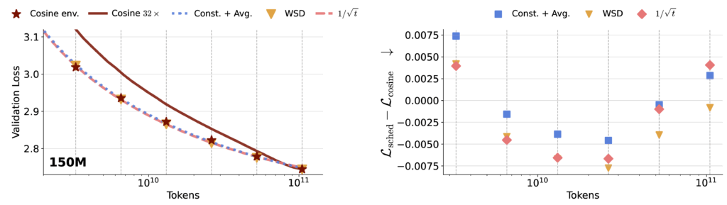
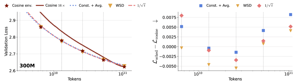
What we observe

• A single long run with constant LR + averaging can closely track cosine across a wide range of horizons.
• A single long run with a $1/\sqrt{t}$-type schedule + averaging is similarly competitive.
• WSD performs well but requires horizon-related decisions (when to start decay).
• In contrast, cosine schedules tuned for one terminal horizon do not reliably transfer to earlier checkpoints.

Theory: anytime $1/t^\gamma$ schedules with averaging

To clarify when horizon-free schedules should work, we analyze SGD on linear regression under spectral assumptions. The key conclusion is that polynomially decaying schedules with tail averaging can match the rates of well-tuned averaged SGD, without requiring knowledge of the horizon.

Informal theorem statement

For SGD run on $N$ samples, a polynomially decaying learning rate of the form $\eta_t = \eta/t^\gamma$ with $0<\gamma<1$, with tail averaging, matches the convergence rates of well-tuned SGD with averaging, where the exponent $\gamma$ depends on spectral properties of the data.

Power-law spectra: optimal $\gamma$

Assume a power-law spectrum and source condition:

• Eigenvalues: $\lambda_i \asymp i^{-a}$
• Signal condition: $\mathbb{E}[\lambda_i (w_i^\star)^2] \asymp i^{-b}$

Then the optimal choice is:

$$
\gamma^\star = \max\left\{1-\frac{a}{b}, 0 \right\}
$$

With $\gamma=\gamma^\star$, the excess risk achieves (up to logs/constants):
$$
\mathcal{R}(w)-\sigma^2 \;\lesssim\; \left(\frac{\sigma^2}{N}\right)^{1-\frac{1}{b}}.
$$

Interpretation:

• If $b \gg a$ (signal concentrated in top eigendirections), more aggressive decay is beneficial (larger $\gamma$).
• If $b \le a$ (signal lives in the tail), constant learning rates with averaging are favored ($\gamma^\star=0$).

WSD through a quadratic lens

WSD consists of a constant phase followed by a linear decay near the end of training. In quadratic settings, decaying learning rates without averaging can be closely related to constant learning rates with averaging: both implement implicit weighting over samples/iterates, but in different ways.

This perspective helps explain why WSD can be competitive in practice while also motivating constant LR + averaging as a simpler, truly anytime alternative.

Practical takeaway: a simple anytime recipe

Our results suggest a pragmatic recipe for horizon-free pretraining:

• Use a simple horizon-free step size (constant or $1/\sqrt{t}$-type).
• Maintain weight averaging (EMA or tail averaging) and evaluate using the averaged weights.
• Tune hyperparameters to do well across checkpoints, not only at one terminal horizon.

Across our 150M and 300M language-model runs spanning large compute ranges, these schedules track cosine closely at intermediate checkpoints without requiring prior knowledge of the final training horizon.

Conclusion

Most standard LLM pretraining recipes are not anytime because they rely on horizon-dependent schedules (notably cosine decay) and are tuned for a fixed compute budget. We propose evaluating anytime behavior against the cosine envelope, and show that simple horizon-free schedules—constant or $1/\sqrt{t}$-type—become competitive with cosine when paired with weight averaging.

On the theory side, in linear regression with power-law spectra, we show that schedules of the form $1/t^\gamma$ with tail averaging achieve optimal rates (up to logs/constants), with the optimal $\gamma$ determined by source and capacity exponents. Empirically, on 150M and 300M LMs trained across large compute multiples, these schedules track cosine closely across training time without requiring horizon knowledge.

Taken together, our results suggest that weight averaging + simple horizon-free step sizes offer a practical and effective anytime alternative to cosine learning-rate schedules for LLM pretraining.