Accelerating RL for LLM Reasoning with Optimal Advantage Regression

Recent LLM advances show the effectiveness of RL with rule-based rewards, but methods like GRPO and PPO are costly due to critics or multiple generations per prompt. We propose a new RL algorithm that estimates the optimal value function offline from the reference policy and performs on-policy updates using only one generation per prompt.

Recent advances in large language models (LLMs), including OpenAI-o1, DeepSeek-R1, and Kimi-1.5, have demonstrated remarkable reasoning capabilities. These models excel at producing long Chain-of-Thought (CoT) responses when tackling complex tasks and exhibit advanced, reflection-like reasoning behaviors. A key factor driving these improvements is reinforcement learning (RL) with rule-based rewards derived from ground-truth answers, where models receive binary feedback indicating whether their final answers are correct.

Substantial efforts have been devoted to refining RL algorithms, such as PPO and GRPO, to further improve performance and training stability. However, these methods either require explicit critic networks to estimate value functions or advantages, or rely on multiple generations per prompt, leading to substantial computational overhead and memory consumption. These limitations make it challenging to scale to long-context reasoning tasks and larger model sizes. This naturally raises the question: Can we develop simpler and more efficient RL algorithms for long context reasoning?

Our answer is $A^\star$-PO, Policy Optimization via Optimal Advantage Regression, a policy optimization algorithm that uses only a single sample per prompt during online RL. Instead of relying on an explicit value network or multiple online generations to estimate the advantage of the current policy during training, our approach directly approximates the fixed optimal value function in an offline manner without a value model.

Figure 1: Prior methods such as GRPO and PPO incur high computational costs, either due to requiring multiple samples per prompt or maintaining an explicit value network. In contrast, $A^\star-PO$ simplifies the training process by estimating the optimal value function using offline generations from $\pi_{\mathrm{ref}}$ and requiring only a single response per prompt during online RL.

Background: Optimal Value Function

Let $x$ denote a prompt (e.g., a math question) and $y$ a generation (e.g., a reasoning chain plus a solution for a given math question). We consider the following KL-regularized RL objective: $$\begin{align*} \max_{\pi} \mathbb{E}_{x, y\sim \pi(\cdot | x)} r(x, y) – \beta \mathrm{KL}(\pi(\cdot | x) \vert \pi_{\mathrm{ref}}(\cdot | x)). \end{align*}$$ where the reward is binary: $r(x, y) = 1$ if $y$ contains the correct answer, and $0$ otherwise.

The optimal policy for this objective is known to be: $$\pi^\star(y|x) \propto \pi_{\mathrm{ref}}(y|x) \exp( \frac{r(x,y)}{\beta})$$ We denote $V^\star(x)$ as the optimal value function of the KL-regularized RL objective above. Under the assumption that the state transitions are deterministic (e.g., autoregressive generation), $V^\star$ has the following closed-form expression: $$\begin{align} \forall x: \; V^\star(x) = \beta \ln {\mathbb{E}_{y\sim \pi_{\mathrm{ref}}(\cdot | x)}}\left[\exp( r(x,y) / \beta )\right]. \end{align}$$ Note that the expectation in $V^\star$ is under $\pi_{\mathrm{ref}}$, which indicates a simple way of estimating $V^\star$: generate multiple i.i.d. samples from $\pi_{\text{ref}}$ and compute the average.

Algorithm: Policy Optimization via Optimal Advantage Regression

$A^\star$-PO is a two-stage reinforcement learning algorithm that separates the estimation of the optimal value function from policy optimization, offering a simple and scalable alternative to traditional actor-critic methods.

Stage 1: Estimating $V^\star(x)$

For each prompt $x$, the algorithm samples $N$ responses $\{y_i\}_{i=1}^N$ from the reference policy $\pi_{\text{ref}}$ and computes:

$$ \hat{V}^\star(x) = \beta \ln \left( \frac{1}{N} \sum_{i=1}^N \exp\left(\frac{r(x, y_i)}{\beta}\right) \right) $$

This can be done offline, using fast inference libraries without any backpropagation, and any off-shelf faster inference library can be used for this stage. It’s fully parallelizable and can optionally filter out hard prompts where all $N$ responses are incorrect.

Stage 2: Policy Optimization via Advantage Regression

With $\hat{V}^\star(x)$ estimated, the algorithm performs online policy updates. Specifically, at iteration $t$, given the current policy $\pi_t$, we optimize the following loss: $$\begin{align*} \ell_t(\pi) := {\mathbb{E}_{x,y\sim \pi_t(\cdot | x)}}\left( \beta\ln \frac{\pi(y|x)}{\pi_{\text{ref}}(y|x)} – \left(r(x,y) – \hat{V}^\star(x) \right) \right)^2, \end{align*}$$ where the expectation is taken under the current policy $\pi_t$ and $r(x,y) – \hat{V}^\star(x)$ approximates the optimal advantage $A^\star(x,y) = r(x,y) – V^\star(x)$ in the bandit setting as $Q(x, y) = r(x, y)$—hence the name $A^\star$-PO. When $\hat{V}^\star(x) = V^\star(x)$, the optimal policy $\pi^\star$ for the KL-regularized RL objective is the global minimizer of the least-squares regression loss, regardless of the distribution under which the expectation is defined (i.e., MSE is always zero under $\pi^\star$). Notably, during this online stage, we generate only a single sample $y$ per prompt $x$, significantly accelerating the training.

The full algorithm is outlined below:

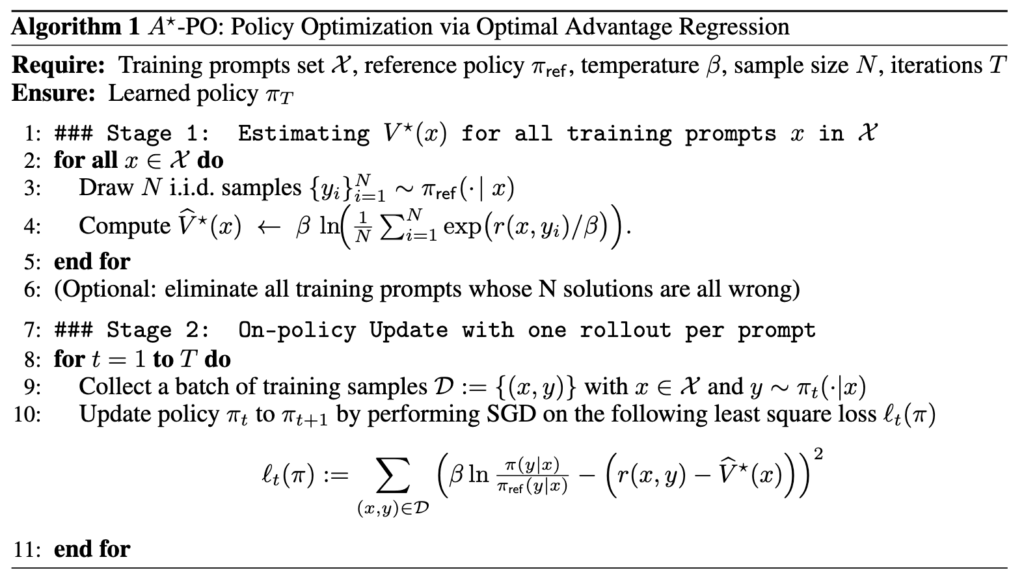
Figure 2: Pseudocode for $A^\star-PO$

Unlike PPO and GRPO, which use clipping and rely on the current policy’s advantage $A^{\pi_t}$, $A^\star$-PO uses a fixed KL regularization to the reference policy and regresses directly on the optimal advantage $A^\star$. This avoids the need for on-the-fly value estimation, multiple rollouts, or critic networks. $A^\star$-PO does not follow the approximate policy iteration paradigm. It places no explicit constraints on keeping $\pi_{t+1}$ close to $\pi_t$. Instead, it directly aims to learn $\pi^\star$ by regressing on the optimal advantages.

Implementation

Our implementation of $A^\star$-PO closely follows the pseudocode above, with the only modification of using two different KL-regularization coefficients, $\beta_1$ and $\beta_2$, during stages 1 and 2, respectively. In stage 1, we employ a relatively large $\beta_1$ to ensure a smoother estimation of $V^\star(x)$. In contrast, a smaller $\beta_2$ is used in stage 2 to relax the KL constraint to $\pi_{\text{ref}}$, encouraging the learned policy $\pi$ to better optimize the reward. Although this introduces an additional hyperparameter, we find that the same set of $\beta_1$ and $\beta_2$ works well across different datasets and model sizes, and therefore, we keep them fixed throughout all experiments.

Faster and More Memory-efficient

We first conduct experiments on GSM8K dataset with 3 different model sizes from Qwen-2.5 family and compare $A^\star$-PO against PPO, GRPO, and REBEL. The results are summarized in the figure below.

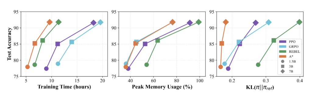
Figure 3: Test accuracy versus training time, peak memory usage, and KL divergence across four baselines and three model sizes on GSM8K. Our approach (orange) can achieve comparable performance (accuracy) to baselines GRPO and PPO, while being 2x faster, more memory efficient, and achieving a smaller KL divergence. Note that for $A^\star-PO$, the training time includes the time from both stages (i.e., offline data collection from $\pi_\mathrm{ref}$ and online RL training).

While all methods achieve similar test accuracy, they exhibit substantial differences in training time, peak memory usage, and KL-divergence. Although REBEL achieves comparable training time as $A^\star$-PO, it requires significantly more memory due to processing two generations simultaneously during each update. GRPO shows similar peak memory usage but requires two generations per prompt and performs twice as many updates as $A^\star$-PO, leading to approximately 2$\times$ longer training time. PPO incurs both higher computational cost and memory usage due to its reliance on an explicit critic.

By consistently updating with respect to $\pi_{\text{ref}}$, $A^\star$-PO maintains the smallest KL divergence to the reference policy. Overall, $A^\star$-PO achieves the fastest training time, lowest peak memory usage, and smallest KL divergence compared to all baselines with similar test accuracy.

Generalizes to Other Benchmarks

One may wonder if explicitly pre-computing $V^\star$ for all training prompts would result in overfitting to the training set. We also conduct experiments on the MATH dataset and evaluate on out-of-domain benchmarks. The results are summarized in the table below.

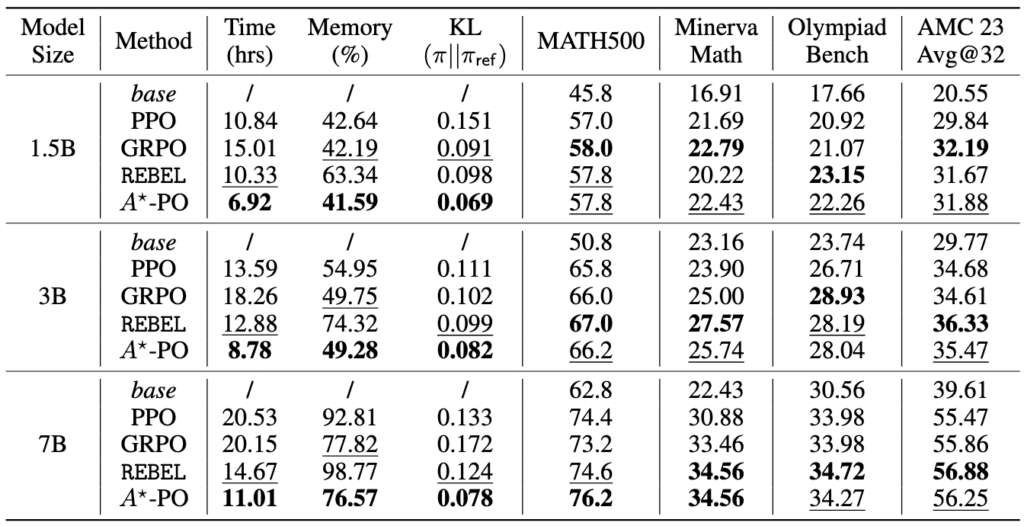
Figure 4: Results on MATH. For each metric, the best-performing method is highlighted in bold, and the second-best is underlined.

For in-distribution test set MATH500, $A^\star$-PO achieves similar performance to baselines on smaller model sizes (1.5B and 3B), but outperforms on the larger model size (7B). When evaluating on the out-of-domain benchmarks, including Minerva Math, Olympiad Bench, and AMC 23, $A^\star$-PO also demonstrates strong generalization capabilities.

Number of Generations for Estimating $V^\star$

To investigate the sufficient number of generations to accurately estimate the value function, we conduct an ablation on the number of generations $N$ used during stage 1 to estimate $V^\star$ on the MATH dataset with the 3B model, varying $N$ from 1 to 32.

Figure 5: Ablation results with different number of $N$ for estimating $V^\star$. Solid lines indicate the moving average with window size 100. (Left) Squared regression loss per step of $A^\star-PO$. (Middle) Training reward per step. (Right) Model performance on MATH500 with varying values of $N$.

We observe that the squared regression loss consistently decreases as $N$ increases, indicating that larger values of $N$ lead to more accurate estimations of $V^\star$. The accuracy of this estimation significantly affects both the training reward and downstream evaluation metrics, such as performance on MATH500. Notably, the training reward increases almost monotonically with larger $N$, and a similar trend is observed for performance on MATH500, which begins to plateau at $N=8$.

More Efficiency by Filtering Out Hard Problems

Since we generate multiple responses for each prompt in stage 1, we could filter out problems whose pass@N is zero to further improve the training efficiency. The intuition is that problems the reference policy $\pi_{\text{ref}}$ is unable to solve (i.e., with near-zero success probability) are unlikely to be solved through RL post-training. Our method naturally supports this filtering mechanism, as we already estimate $V^\star$ during the offline stage. We conduct an ablation study varying $N$ from 2 to 32, filtering out problems where all $N$ sampled responses are incorrect.

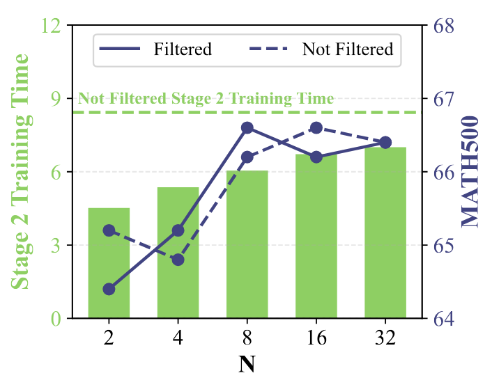
Figure 6: Ablation Results on Filtering Hard Prompts. (Green) Training time of Stage 2 for different values of $N$. The dashed line indicates the training time without filtering. (Purple) Performance on MATH500 with and without filtering.

Filtering significantly reduces training time by reducing the effective size of the training set, as illustrated by the green bars compared to the dashed baseline. When $N$ is small, filtering removes more problems since it is more likely that none of the $N$ responses are correct, further accelerating training. In terms of performance, the MATH500 evaluations for filtered and unfiltered runs remain closely aligned. Notably, the filtered run with $N=8$ achieves the highest accuracy, even surpassing the unfiltered baseline while reducing training time by 28\%.

Optimal $\beta_1$ for Estimating $V^\star$

The parameter $\beta_1$ controls the level of smoothness when estimating $V^\star$. As $\beta_1 \to 0$, the estimated $V^\star$’s value approaches Pass@N (computed using the collected $N$ responses), while as $\beta_1 \to \infty$, it estimates $V^{\pi_{\text{ref}}}$. We ablate $\beta_1$ from $\infty$ to $1/8$ to investigate the optimal value.

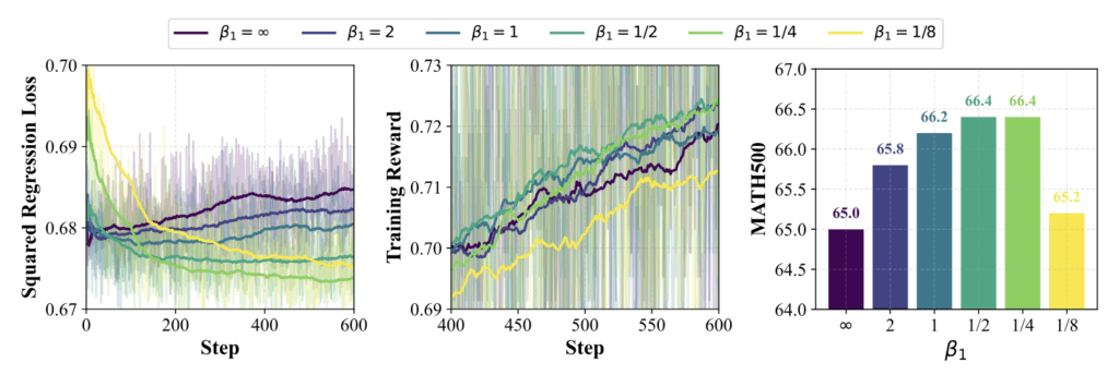
Figure 7: Ablation results with different $\beta_1$ for estimating $V^\star$. Solid lines indicate the moving average with window size 100. (Left) Squared regression loss per step of $A^\star-PO$. (Middle) Training reward per step. (Right) Model performance on MATH500 with varying values of $\beta_1$.

From the squared regression loss, we observe that smaller values of $\beta_1$ lead to higher initial training loss. But the final training loss decreases monotonically as $\beta_1$ decreases, until reaching $\beta_1 = 1/8$. A similar trend is observed for both the training reward and MATH500 performance, which improve monotonically with smaller $\beta_1$ values up to $\beta_1 = 1/8$. Further decreasing $\beta_1$ may produce an overly optimistic estimate of $V^\star$, which the model cannot realistically achieve, ultimately hindering performance.

Near-optimal Without Sophisticated Exploration

$A^\star$-PO not only simplifies RL training but also comes with strong theoretical guarantees—achieving near-optimal performance without any sophisticated exploration.

Traditional RL algorithms often require active exploration (e.g., entropy bonuses) and strong structural assumptions such as policy completeness. In contrast, $A^\star$-PO provably converges to a near-optimal policy under much weaker conditions: – The policy class is realizable, and the loss function is bounded. – The reference policy $\pi_{\text{ref}}$ must have non-zero success probability (e.g., pass@k > 0) on each prompt.

Using tools from no-regret online learning and bandit theory, $A^\star$-PO’s performance gap to the optimal policy $\pi^\star$ shrinks at a polynomial rate with respect to the number of training iterations. This result holds for general policy classes and even for high-dimensional log-linear models, without requiring bi-level optimization or token-level exploration.

In short, $A^\star$-PO learns near-optimal policies efficiently—without exploration, critics, or complex algorithms.

Conclusion

We introduced $A^\star$-PO, a simple yet powerful policy optimization algorithm tailored for reasoning tasks with large language models. By separating value estimation (offline) and policy learning (online), and regressing on optimal advantages rather than estimating policy-specific ones, $A^\star$-PO:

• Eliminates the need for critics and multiple generations per prompt
• Achieves state-of-the-art efficiency in both training time and memory
• Generalizes well to both in-domain and out-of-domain reasoning benchmarks
• Offers strong theoretical guarantees