InputDSA: Demixing then comparing recurrent and externally driven dynamics in complex systems

We explored how to measure the similarity between two complex systems when they are driven by external inputs, like biological neural circuits or reinforcement learning agents. Our novel method, called InputDSA, disentangles each systems’ intrinsic dynamics from its input-driven effects, enabling highly accurate, robust, and efficient comparisons of those components.

This blog post is based on work done with Mitchell Ostrow, Satpreet Harcharan Singh, Leo Kozachkov, Ila Fiete, and Kanaka Rajan. This work has been accepted to ICLR 2026.

Comparing different systems to reveal the structure of emergent computations

Across fields like deep learning and computational neuroscience, identifying similarities among complex systems is crucial for understanding their emergent computations. Whether we are comparing different artificial neural networks, analyzing activity across brain regions and stages of learning, or evaluating how well computational models capture biological mechanisms, we face a central question: how do we know when two disparate systems share the same underlying structure, and how do we choose the right comparison method to capture the specific computations we care about?

One common approach to characterizing the similarity of two systems is to compare the geometry of their internal states. Well-known methods for capturing and comparing this geometric structure include Representational Similarity Analysis, Centered Kernel Alignment, Procrustes Analysis, Canonical Correlation Analysis, and Pearson Correlation. However, in most physical systems, including the brain and time-varying neural networks, computation unfolds over time. To capture these temporal dynamics, tools like Dynamical Similarity Analysis (DSA) offer an important alternative. DSA provides an efficient, theoretically grounded metric that measures the similarity of recurrent dynamics over time rather than just geometric shape at a snapshot moment. 

Yet, DSA relies on a major assumption: that a system evolves autonomously. However, most systems of interest in neuroscience and machine learning are non-autonomous, receiving sensory signals or communication from other subsystems. They are driven by complex external inputs and can receive observations that are contingent on the systems’ outputs. When activity is the result of both intrinsic dynamics and input drive, comparisons can be confounded by inputs.

To bridge this gap, we introduce InputDSA. This novel method explicitly disentangles a system’s intrinsic dynamics from its input-driven effects. By estimating both the internal state-transition operator and the input-to-state mapping, InputDSA enables highly accurate, robust comparisons of these components, either jointly or independently, offering a powerful toolkit for comparing real-world, non-autonomous systems. 

Input-aware Dynamical Similarity Analysis (InputDSA)

At a high level, comparing two complex, input-driven systems requires two distinct steps. First, we must extract both the underlying intrinsic and input-driven dynamics of each system from its states and inputs over time. Second, we must mathematically compare those extracted dynamics across systems to see how similar they are. Let’s walk through each step.

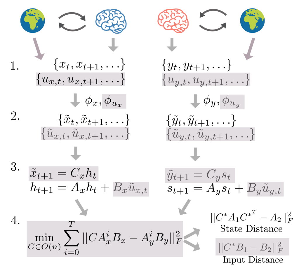
Step 1: Estimating the Linear Operators

Consider a linear, input-driven dynamical system whose state evolution can be written as

$$\dot{x} = A x + B u(t)$$

In this setup, the $A$ matrix represents the system’s intrinsic dynamics—how its internal states evolve autonomously. The $B$ matrix represents the input-to-state mapping—how external inputs $u(t)$ are injected into the system.

The original DSA framework relies on Dynamic Mode Decomposition (DMD) to fit a linear operator to autonomous dynamics:

$$\phi(x_{t+1}) = A\phi(x_t)$$

The goal of the DMD is to approximate the Koopman Operator (Koopman, 1931), a theoretical object that exists for all dynamical systems, which encodes the linear dynamics of observables (functions that act on the true system state) under the system dynamics. Here, $\phi$ is a nonlinear embedding of the data that typically expands the dimensionality of the state space. Intuitively, the dimensionality expansion acts similarly to the kernel trick, where embedding into higher dimensions ‘unfolds’ the nonlinearity. For systems that are driven by external inputs, a natural extension to DMD is DMD with control (DMDc):

$$\phi_1(x_{t+1}) = A\phi_1(x_t) + B\phi_2(u_t)$$

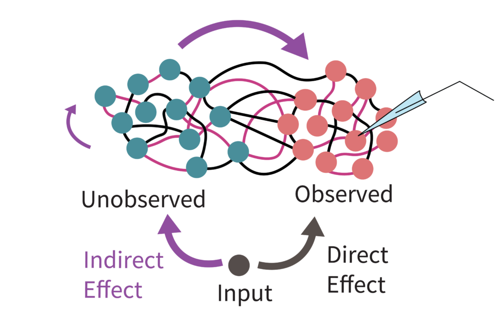
While separately estimating A and B via DMDc is an intuitive extension to input-driven systems, it suffers from a hidden failure mode in practice: partial observation. In fields like neuroscience, we usually only record a small fraction of a vast neural population. When an external input enters the circuit, it drives both our recorded neurons, and the unobserved neurons. Those unobserved neurons then pass the signal back into our recorded subset through their recurrent connections. Since the algorithm doesn’t “know” there are unobserved neurons, it gets confused by this indirect routing and misinterprets these delayed internal echoes as the direct effect of external inputs. Consequently, the system’s intrinsic dynamics get mixed into the input-driven dynamics, causing our estimate of the input mapping ($B$) to become heavily biased by the internal rules ($A$) (Fig. 2).

To mitigate this problem, we introduce Subspace DMDc, which explicitly separates a system’s observed states from the hidden, latent states that dictate its full evolution over time. In brief, Subspace DMDc utilizes subspace identification algorithms from classical control theory, which seek to identify linear dynamical systems of the form:

$$x_{t+1} = A x_t + B u(t)$$

$$y_t = C x_t$$

Here, only the outputs ($y_t$) and the inputs ($u_t$) are actually observed.

Step 2: The Similarity Metric

Now that we have accurately estimated $A_1, B_1$ for the first system and $A_2, B_2$ for the second, how do we compare them?

A key feature of input-driven systems is their controllability: the ability of an input sequence to steer the system’s state to arbitrary points over time. In our linear approximation, this cascading effect of the input is elegantly captured by the $T$-step controllability matrix:

$$K_1(T) = \begin{pmatrix} B_1 & A_1B_1 & A_1^2B_1 & \dots & A_1^{T-1}B_1 \end{pmatrix}$$

Intuitively, this matrix traces how a signal enters the system ($B_1$) and then cascades through the recurrent connections step by step ($A_1B_1$, $A_1^2B_1$, etc.). It encodes the geometric space of all the directions the input can push the system.

Crucially, the geometric properties of this controllability space are preserved if we simply rotate or flip the coordinate system via an orthogonal transformation ($C$). If two systems are truly implementing the same underlying computations, their controllability matrices should match up once they are properly aligned. This motivates our proposed similarity metric, InputDSA. We search for the optimal rotation $C$ that minimizes the difference between the two systems’ controllability matrices:

$$\text{InputDSA} = \min_{C \in O(n)} ||CK_1 – K_2||^2_F$$

Because this takes the form of a classic Procrustes alignment problem, we can solve it highly efficiently. Once we find the optimal alignment $C^*$, we can split the unified distance back apart to study the intrinsic and input-driven components independently:

$$\text{InputDSA}_{\text{state}} = ||C^*A_1C^{*^T} – A_2||_F^2$$

$$\text{InputDSA}_{\text{input}} = ||C^*B_1 – B_2||_F^2$$

InputDSA discriminates intrinsic from input-driven dynamics, and is robust to partial observation

To demonstrate that InputDSA can capture similarities in both intrinsic and input-driven dynamics, we construct four sets of partially observed random RNNs driven by low-pass filtered white noise. We engineered these networks so that Systems 1 and 2 (as well as 3 and 4) share the same intrinsic dynamics, while Systems 1 and 3 (as well as 2 and 4) share the same input effect (Fig. 3A). Each system has 20 dimensions, but only two are observed. 

Here, the ground-truth distance matrix between all systems for their intrinsic dynamics (the “state distance”) should exhibit a block-diagonal structure, with low distances on the diagonal and high distances off-diagonal. Meanwhile, the distance matrix for the input-driven dynamics (the “input distance”) should show a checkerboard structure. We found that while standard DMD and DMDc captured some of the true state similarity structure, the SubspaceDMDc similarity scores were noticeably sharper (Fig. 3BC).

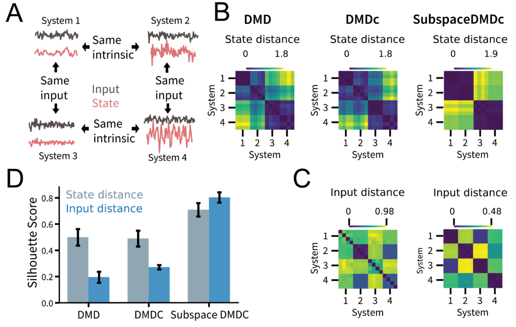
Repeating this same experiment across 100 random seeds and quantifying how well we could separate and cluster the different systems based on the distance matrices estimated by each method, we found that SubspaceDMDc consistently yielded the best separability, represented by a higher Silhouette score (Fig. 3D).

InputDSA is robust to partial observation

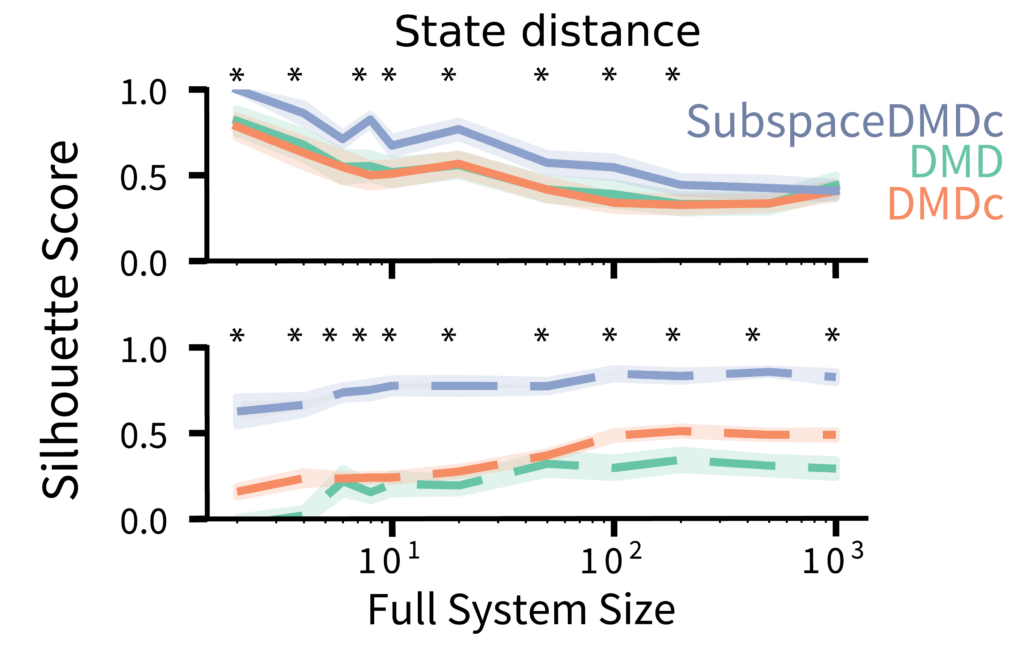
To assess the effect of partial observation, we ran the above analysis for systems of varying sizes (ranging from 2 to 1,000 dimensions) while persistently observing only 2 dimensions. As the total system size increased (therefore became less observed), the state similarity scores for each method gracefully degraded, though SubspaceDMDc maintained a noticeable improvement over the other methods. For the input-driven dynamics, although the DMDc input score never appeared robust, the SubspaceDMDc input similarity remained highly robust across all system sizes (Fig. 4).

InputDSA identifies how successful and unsuccessful agents differ over training

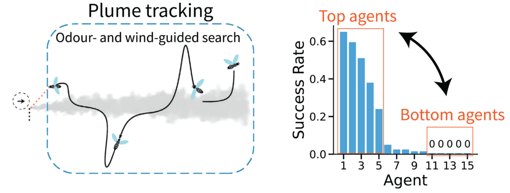
In closed-loop Reinforcement Learning (RL) environments, stochasticity in action sampling can shift the input distribution across training, leading to drastic divergences in agent behavior later on. The Plume Tracking task exhibits substantial behavioral variability (Fig. 5). In this environment, artificial flies (RNNs) trained via deep RL must navigate a simulated windy arena to locate the source of an odor, requiring them to constantly balance memory-based intrinsic dynamics with rapid, stimulus-driven responses.

This raises a key question: when some agents succeed, and others fail, is the performance gap driven by differences in their intrinsic memory, or by their input-driven responses to wind and odor concentration? Applying InputDSA revealed that the input-driven dynamics of the highest-performing (“Top”) agents cleanly separated from those of the failing (“Bottom”) agents, whereas their intrinsic dynamics showed no significant difference (Fig. 6A). By further analyzing the input-mapping operator ($B$), we found that in successful agents, external inputs consistently exert a stronger, more direct effect on the recurrent dynamics—characterized by a more slowly decaying singular value spectrum (Fig. 6B). This indicates that successful tracking relies heavily on robust, input-driven computations rather than internal memory.

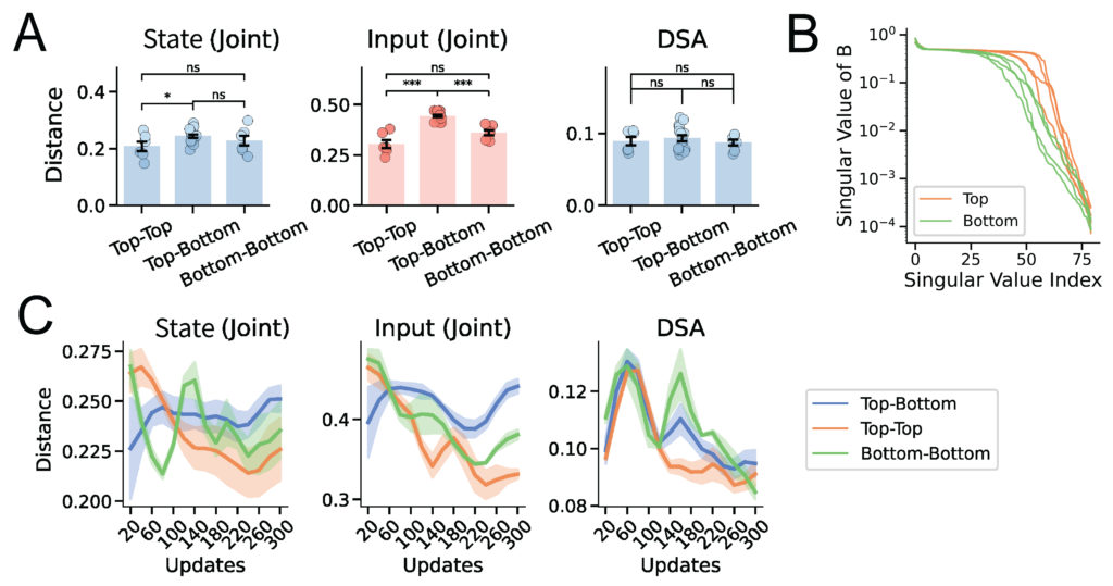
Tracing individual variability in neural dynamics over training, we found that while within-group input similarity decreases over time for both the Top and Bottom agents, the Top agents ultimately converge to a much more consistent set of input-driven dynamics. The Bottom agents, in contrast, diverge toward heterogeneous, idiosyncratic dynamics (Fig. 6C). It is a neat computational example of Tolstoy’s famous “Anna Karenina principle”: every successful agent is alike, but every failing agent fails in its own way.

InputDSA captures differences in neural population dynamics over task epochs

We also applied InputDSA to a recently published dataset in which neural population activity was recorded from six frontal and striatal regions during an auditory evidence accumulation task. During the task, rats were trained to listen to auditory pulses from either side and turn toward the side with more pulses (Fig. 7A). In the original study, the authors defined the neural time of commitment (nTc) as the internal moment during perceptual decision-making when an animal has effectively committed to a choice (Fig. 7B).

To examine how neural population dynamics reorganize across this critical point, we applied InputDSA to neural activity before and after the nTc. Here, we constructed the external inputs as two-dimensional time-series encoding the number of left and right auditory pulses within each time bin. InputDSA revealed a significant shift in both the intrinsic and input-driven dynamics across the commitment point (Fig. 7C), consistent with the changes reported by Luo et al. (2025).

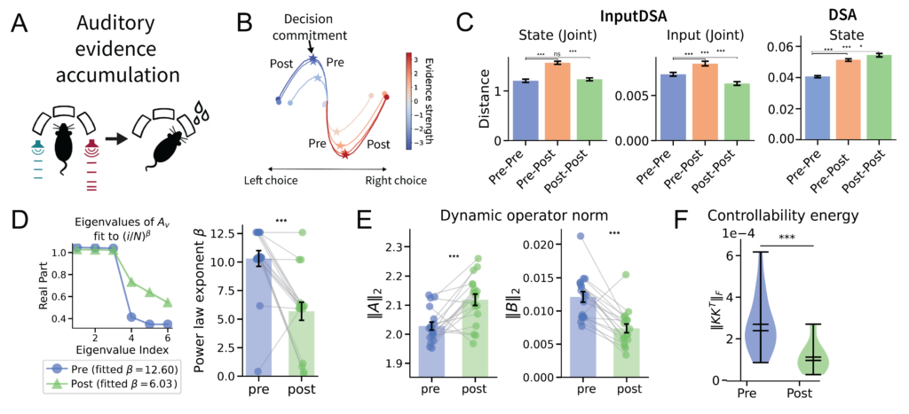
Comparing the eigenspectrum of the state-transition matrix $A$ before and after the nTc, we found that post-commitment periods consistently exhibited a more slowly decaying eigenspectrum, indicating longer-lasting intrinsic dynamics (Fig. 7D). Conversely, pre-commitment periods featured a faster decaying eigenspectrum with a higher density of small eigenvalues. Smaller eigenvalues in the $A$ matrix imply greater input controllability, characteristic of a highly input-driven system—aligning with the pre-nTc regime identified by Luo et al. (2025). Likewise, the average magnitude of the intrinsic dynamics strengthened while the input-driven dynamics weakened in the post-nTc period, reflecting a transition into a more autonomous, less input-sensitive regime(Fig. 7E).

Lastly, we computed the Frobenius norms of the controllability Gramians ($||KK^T||_F$) before and after the nTc, which measure how easily the system can be steered into arbitrary directions in state space. The distribution of norms decayed significantly across the nTc ($p < 0.001$, Mann-Whitney U-test), confirming that the neural dynamics become less input-controllable over time (Fig. 7F).

Together, these results demonstrate that population activity undergoes a fundamental regime change at the nTc: transitioning from an input-driven, evidence-accumulation phase into an intrinsically dominated, decision-commitment phase, consistent with by Luo et al. (2025).

Summary and Future Impact

We introduced InputDSA, a theoretically grounded method to quantitatively compare both the intrinsic dynamics and the effects of external inputs between two dynamical systems, based on data alone. While our current study applied InputDSA to biological neural data and recurrent neural networks, InputDSA can easily be applied to any time-series data.

Looking ahead, InputDSA opens several exciting avenues for future research. It could be used to:

• Enable accurate comparisons in complex, input-driven dynamical systems. This includes evaluating different RL agents, analyzing multi-area interactions across different brain regions, or comparing neural activity across animals and different behavioral contexts.
• Uncover underlying similarities in naturalistic, real-world settings where external inputs are noisy or not perfectly controllable, e.g., neural dynamics in naturalistic neuroscience tasks. 
• Validate models via causal perturbation: Validate computational models against biological circuits using causal perturbations (such as optogenetic or electrical stimulation). This provides a much more stringent test than comparing intrinsic dynamics alone.
• Design optimal inputs: Facilitate optimal input design to drive neural dynamics maximally apart in their state space.

Finally, InputDSA is highly accessible and computationally efficient. For a reasonably sized system (e.g., 50 dimensions and 10,000 timepoints), the method takes about sixty seconds to fit on a standard laptop (tested on an M1 Pro Mac), and it scales even faster when run on a GPU.