Flow Equivariant Recurrent Neural Networks

Sequence transformations, like visual motion, dominate the world around us, but are poorly handled by current models. We introduce the first flow equivariant models that respect these motion symmetries, leading to significantly improved generalization and sequence modeling.

Introduction

As you aimlessly gaze out the window of a moving train, the hills in the distance gently flow across your visual field. Without even trying, you recognize trees swaying in the breeze and cows grazing on the grass. This effortless ability to understand scenes despite their motion is a hallmark of representational structure with respect to motion — a type of structure that today’s best sequence models still lack. 

Take for example the scene of two handwritten numbers (4 and 0) slow drifting across a black background presented below:

Figure 1: Comparison of the feature maps for RNNs trained on a ‘Moving MNIST’ next-step prediction task. We see that the Flow Equivariant model has much more coherent representations of the image despite the ongoing motion.

On the top row, we show four feature maps from the hidden state of a (convolutional) recurrent neural network, and the motion-stabilized versions to the right. As we can see, the feature maps begin to lose coherent structure as time goes on. This lack of structure is more than just intuitively unpleasing, it implies a fundamental inconsistency in how the RNN has learned to model motion and sequences. Below, we show the corresponding feature maps for our newly introduced Flow Equivariant Recurrent Neural Network (FERNN) — the first known sequence model which represents motion in a properly structured manner. As can be seen, these models maintain structure in their hidden state with respect to motion over extended timespans; and, as we will show, this yields large improvements to training speed and generalization on datasets with significant motion.

In the following, we will give a brief review of equivariance, an overview of how we built this model, the quantitative results, and the potential implications for neuroscience. For the full paper, please check out our preprint and our code on GitHub.

‘Static’ Equivariance

An equivariant deep neural network is simply one that processes transformed data in ‘the same way’ that it processes untransformed data, but with a corresponding structured transformation in its output (in other words, it is different than being ‘invariant’ to the transformation). This property ensures that no matter how your data arrives, the model will always handle it in a consistent pre-specified manner which makes it easily relatable to the untransformed data. 

The most well known example of an equivariant network is the convolutional neural network, which is equivariant with respect to spatial shifts (a.k.a. the translation group). This translation equivariance is arguably what led to the success of convolutional neural networks, and the ultimate resurgence of deep neural networks broadly in the early 2010’s.

One way to verify equivariance is to check that the order in which the transformation and the neural network are applied to the data does not change the result (formally, the transformation and the feature extractor commute). If we call the data $\mathbf{x}$, the neural network $f$, and the transformations of the input and output spaces $\tau_g$ and $T_g$ respectively, then we get the following equivariance relation: $T_g[f(\mathbf{x})] = f(\tau_g[\mathbf{x}])$, visualized below.

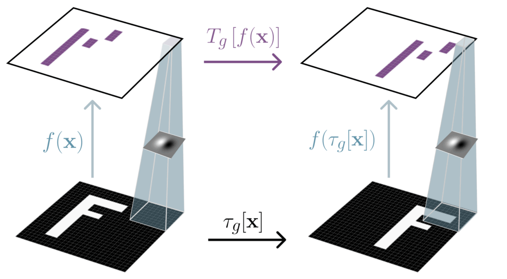
Figure 2: A convolutional neural network $f$ is equivariant to translations of the input ($\tau_g[\mathbf{x}]$), meaning that the output $f(\mathbf{x})$ also shifts when the input shifts.

As can be seen, for convolution, the input and output transformations are the same (both are spatial shifts). However, if we want to be equivariant to more complex groups such as the group of 90-degree rotations (and spatial shifts), as in Group Equivariant Convolutional Networks (Cohen & Welling, 2016), the output space transformation $T_g$ can get a bit more complicated. In the construction visualized below, $T_g$ is actually a spatial rotation and a permutation of a new ‘lifted’ rotation channel dimension. The extra channel permutation and ‘lifted’ dimension are indeed necessary to represent this more complex group.

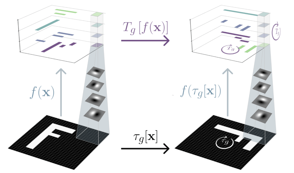
Figure 3: A $p4$ group equivariant convolutional neural network is equivariant to 90-degree rotations of the input, meaning that when the input rotates, its output rotates spatially in unison, but the channels also cyclically permute through the ‘lifted’ rotation dimension (shown vertically).

To date, equivariant neural networks have been developed for a wide range of transformations from 3D-rotations, to scale transformations, to any continuous Lie Group. These networks have demonstrated huge benefits for data that contains many of these transformations, and are now the default inductive bias of choice for scientific data applications. Notably, however, the transformations considered have been restricted to those which are static with respect to time; such as the rotation or translation of the image F above, or the 3D rotation of a molecule before training a diffusion model on it.

While these types of transformations have been sufficient for the past decade of feed-forward convolutional neural networks, as we now enter the age of large language models, video diffusion models, and world modeling, there is a new class of data that has risen to center stage, and with it a new class of transformations — namely, sequence data and sequence transformations. 

Equivariance for Sequence Data — “Flow Equivariance”

In this work, we introduce a new type of equivariance for these sequence transformations which we call ‘Flow Equivariance.’ A flow is a mathematical object which can informally be thought of as a constant velocity transformation parameterized by time. Flows can be rotations, scaling, shearing, 3D rotation, etc, each slowly and continuously progressing over time. For example, if I am walking down the street with velocity $\nu$, my position over time can be described as $x_t = x_0 + \nu t$, for a starting position $x_0$. This addition operation can equivalently be thought of a ‘flow,’ a time-parameterized transformation, acting on my position: $\psi_t(\nu)[x_0] = x_0 + \nu t$.

So then, what is flow equivariance? Recalling that we can describe a standard ‘static’ equivariant neural network as one where ‘when the input is transformed, the output has a corresponding structured transformation,‘ we can extend this same definition to apply to sequence transformations and sequence models. In other words:

Flow equivariance is the property of a sequence model such that when the input sequence undergoes a constant velocity transformation over time, the sequence of outputs of the model also has a corresponding structured transformation over time.

This property can be seen to be the same as the idea that the order of feature extraction and transforming doesn’t matter, i.e. if I compute some outputs for an observed sequence $f_t$ in a motionless setting (call the outputs $h[f]$), and then I separately compute some outputs for an observed sequence in motion, $\psi_t(\nu) \cdot f_t$ (call these output $h[\psi(\nu) \cdot f]$), then the two sequences of outputs $h[f]$ and $h[\psi(\nu) \cdot f]$ should be related by a corresponding ‘motion’ in the output space: $\psi(\nu) \cdot h[f] = h[\psi(\nu) \cdot f]$.

As an intuitive example, if the input to my recurrent neural network is a video of a bump moving across the screen from left to right, the hidden states of my recurrent neural network should also have a corresponding structured motion. As we will see in the next section, this intuitive example of flow equivariance does not hold for standard recurrent neural networks, and is also actually violated by the vast majority of modern sequence models including state space models and transformers.

Existing Sequence Models are not Flow Equivariant

To formalize the example above, consider a simple recurrent neural network with identity encoders and non-linearities such that the entire network is described as: $h_{t+1} = h_t + f_t$ for hidden state $h_t$ and input $f_t$. This network can be seen to simply integrate information over time by summing it together, and is a special case of the more general simple recurrent neural network (often written as $h_{t+1} = \sigma(\mathbf{W} h_t + \mathbf{U} f_t))$.

In the figure below, we demonstrate visually that when the input is a single bump, either static (left) or moving (right), the outputs of the network are not relatable by a corresponding motion in the latent space. Instead, what we see is that in the static case, the network performs the expected integration of the signal, yielding a bump that slowly grows larger. Conversely, in the moving case, we see that the hidden state at each time-step is ‘lagging behind’ the new input, causing the input to be added to a different location of the hidden state than the previous bump, and yielding a ‘ghosting’ like effect in the hidden state outputs. As is visually apparent, these two output sequences are not related by a simple sequence motion transformation of the output. 

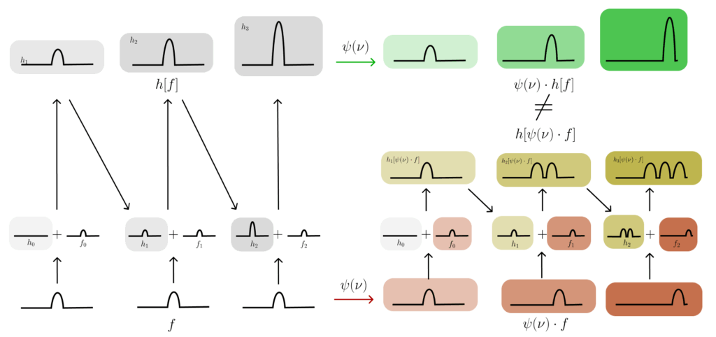
Figure 4: A simple ‘bump input’ example demonstrating that the basic RNN ($h_{t+1} = h_t + f_t$) is not equivariant with respect to movement of the bump, i.e. it is not ‘flow equivariant.’

How to Build Flow Equivariance

How can we then build recurrent neural networks which do satisfy this property? Intuitively, we want to fix the problem that we can clearly see in the figure above; specifically, the fact that the hidden state is ‘lagging behind’ the input by exactly one time-step when the input undergoes a transformation. To accomplish this, we therefore propose to simply augment the hidden state update with an additional shift: $h_{t+1} = \mathrm{shift}_1[h_t] + f_t$. We visualize this new recurrent update below on the same bump example.

Figure 5: The same moving bump example, but with the flow-equivariant update equation ($h_{t+1} = \mathrm{shift}_1[h_t] + f_t$) shows that the RNN is now equivariant to motion.

As can be seen, with this new recurrence, the hidden state is now in-line with the input at each time-step, and the outputs are simply shifted copies of one-another. Another way to understand this difference is that the hidden state is actually being updated in the same moving reference frame as the input. This is clear from understanding that the moving version of the input is actually formed by the same shift operator: $f_{t+1} = \mathrm{shift}_1[f_{t}]$.

However, what we can also see from this example, is that this model is only equivariant with respect to a single velocity, specifically a velocity of 1 shift per time-step. How can we extend this to yield equivariance to multiple velocities simultaneously?

Flow Equivariance for Multiple Velocities

One simple solution to achieve equivariance to multiple velocities is to mirror the construction of Group Equivariant Convolutional Networks. Specifically, we can create multiple copies of our hidden state in separate channels which we call a ‘lifted dimension’, and then apply a separate velocity shift to each one of those channels separately. For example, our previous simple network from before would be given an additional ‘lifted’ velocity index $\nu$, and could be written as: $h_{t+1}(\nu) = \mathrm{shift}_\nu[h_t(\nu)] + f_t$.

In the figure below, we visualize this new multi-velocity flow-equivariant RNN, and see that indeed, the same equivariance property holds, but with a new representation of the transformation in the output space. Similar to the rotation equivariant networks depicted at the start of this article, the transformation on the outputs is now a spatial shift and a shift of the lifted channel dimension.

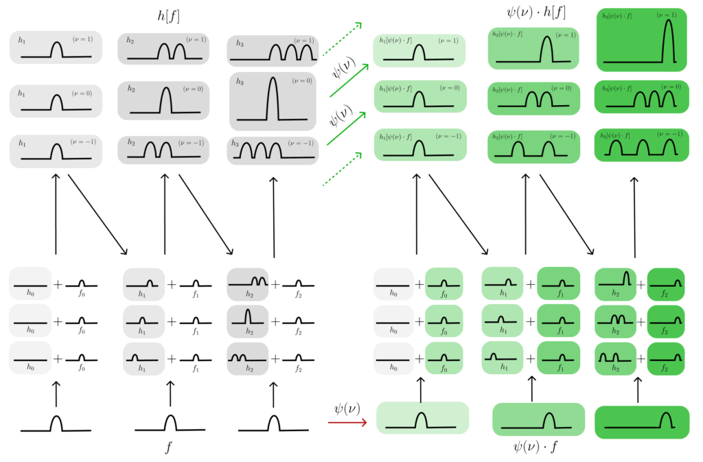
Figure 6: To make the flow-equivariant RNN equivariant to multiple velocities simultaneously, we add multiple different velocity channels, each shifting by a different amount at each timestep.

Formally, we can write the representation of this action as:
$$
\begin{align}
h_t[\psi(\hat{\nu}) \cdot f] (\nu, g) & = (\psi(\hat{\nu}) \cdot h[f])_t(\nu, g) \\
& = h_t[f](\nu – \hat{\nu}, \psi_{t-1}(\hat{\nu})^{-1} \cdot g)
\end{align}
$$

Meaning that when a flow is applied to the input (left hand side) this is equivalent to a flow acting on the output (right hand side), where the action of that flow on the output is given by a spatial shift ($\psi_{t-1}(\hat{\nu})^{-1} \cdot g$), and a shift of the lifted velocity channels ($\nu – \hat{\nu}$). We call this model a Flow-Equivariant RNN (FERNN).

Results

Equivariant neural networks are known to perform better than non-equivariant counterparts when the data they are being applied to contains the same transformations (also called symmetries) to which they are made equivariant. For example, convolutional neural networks (CNNs) perform better than fully connected networks on datasets of images where it is known that the location of the object in the frame is likely to be spatially shifted around. In this paper, we therefore explore the performance of Flow Equivariant RNNs on sequences which contain significant motion transformations — such as MNIST with translation and rotation motions (depicted in the opening video), and a simple video ‘action recognition’ dataset where we augment it to simulate camera motion.

FERNNs Learn Faster

On moving and rotating MNIST datasets, we train the model to observe the first 10 frames of the sequence, and then sequentially generate the next 10 frames of the sequence. What we see is that the FERNN models learn orders of magnitude faster and ultimately reach significantly lower reconstruction error than their non-flow-equivariant counterpart (the regular group-equivariant RNN ‘G-RNN’).

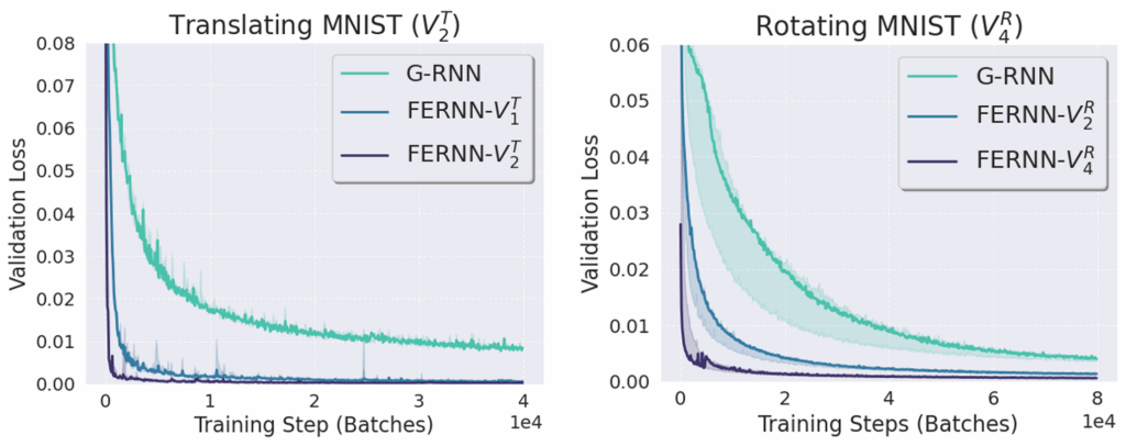
Figure 7: Validation loss over training iterations for convolutional RNNs (‘G-RNN’) and FERNN models trained on a moving MNIST next-step prediction task.

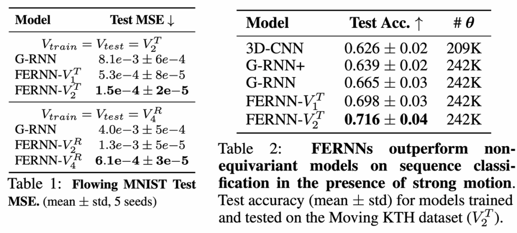
FERNNs Generally Predict and Classify better for data with flow symmetries

We see that across both datasets, FERNNs with more equivariance built in (as denoted by the trailing $V^*_N$ notation) always outperform non-flow-equivariant counterparts on both forward prediction (MNIST, left) and sequence classification (KTH, right).

FERNNs Generalize to longer sequences

One of the most intriguing properties of FERNNs is that they appear to automatically generalize to significantly longer sequences than the non-equivariant counterparts. Specifically, for next-step prediction on moving MNIST videos, the FERNN was able to accurately predict sequences up to 70 timesteps into the future, while only being trained to predict up to 10. Comparatively, we see the non-equivariant counterparts begin to lose coherence with the ground truth shortly after the training length, and coherent structures in the reconstructed image begin to degrade. 

Figure 8: Visualization of the next-step predictions of the FERNN and Convolutional RNN (G-RNN) on moving MNIST (left). We see the FERNN generalizes significantly further than the non-equivariant counterpart. This is also quantitatively shown by the average error w.r.t. Forward prediction timestep in the plot on the right.

FERNNs Generalize to unseen velocities

In addition to the length generalization property, we also see that FERNNs have zero-shot generalization abilities to new velocities not seen during training, but which are built into the network architecture (e.g. though the extra velocity channels we described above). In the figures below, we show that this is the case for both moving MNIST and rotating MNIST, where the FERNN achieves virtually zero error on velocities outside the training range, while the non-equivariant counterpart achieves no such generalization. Intuitively, this generalization property can be understood to arise from the fact that the FERNN effectively shares recurrent parameters between all built-in velocities simultaneously.

Figure 9: Visualization of next-step predictions for high-velocity translations not seen during training. We see the FERNN can model these perfectly, since they are built into the model, while the non-equivariant counterpart cannot. This is again shown qualitatively by measuring the error across the entire test set for each velocity on the right. The training range is depicted by the red bounding box.

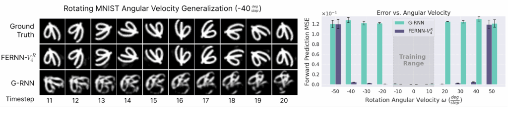
Figure 10: Visualizations of the next-step predictions for high-velocity rotations not seen during training (left), along with their corresponding average error as a function of angular velocity (right). We again see the FERNN generalizes nearly perfectly, while the non-equivariant model does not.

Conclusion

In this paper we introduce a new type of equivariance for sequence models and corresponding sequence transformations. Given the tremendous rise in the popularity of sequence models today, we believe that exploiting the extra symmetries present in these sequences, emerging from the addition of the time dimension, can yield tremendous benefits to model training efficiency and generalization performance, and therefore should be leveraged if at all possible.

Given that biological neural networks are highly recurrent and inherently embodied in a ‘sequence modeling’ setting, we also think that this theory and framework has particularly interesting implications for biological systems. Specifically, prior work has studied the relationship between traveling waves and equivariance in recurrent neural networks, inspired by traveling waves of activity observed to propagate across cortex. Somewhat incredibly, the emergent waves in these models can be seen to be exactly equivalent to the hidden state flows introduced in the FERNN. This equivalence also extends to other traveling wave models where waves were demonstrated to improve long short-term memory in recurrent neural networks. We therefore believe that the FERNN framework may be a way of formalizing the relationship between spatiotemporal neural dynamics and equivariance; and in future work, we intend to explore this connection more thoroughly in both biological and artificial systems.