Where Do Features Come From?

The Mystery

Suppose it is 9am. What will the time be 5 hours from now?

There are many valid ways to solve this problem. For instance:

1. Counting up by one hour five times: 10am, 11am, 12pm, 1pm, 2pm. (At the fourth step, you needed to use the memorized fact that 1, not 13, follows 12 on a clock.)
2. Addition followed by subtraction: 9 + 5 = 14. 14 − 12 = 2. So: 2pm.
3. Memorization: You conveniently remember off the top of your head that 5 hours after 9am is 2pm.
4. Clock visualization: You envision an analog clock set to 9 o’clock in your mind’s eye, and mentally rotate the hour hand five hours forward. At its new angle, you observe the hand is pointing at 2 o’clock.

It would be straightforward to write code implementing any of the above algorithms for modular addition (in this case, adding two integers modulo 12). But this is going to be a story about deep learning, and the fundamental principle of deep learning is laziness: why intelligently design an algorithm and hand-code it yourself, when you could just feed a bunch of data into an off-the-shelf neural network, train it with an all-purpose optimizer, and watch it learn its own computational strategy?

Admittedly, the machinery of deep learning isn’t particularly practically useful for clean, synthetic tasks like this; it’s meant for messy tasks like predicting the next word in Internet text or classifying cats and dogs. But our goal will be understanding deep learning, and scientific understanding is sometimes easiest to arrive at by studying toy cases.

In any case, training a neural network to perform modular addition turns out to be an interesting exercise. In 2022, Power et al. trained transformers on modular arithmetic tasks and observed that, surprisingly, “long after severely overfitting, validation accuracy sometimes suddenly begins to increase from chance level toward perfect generalization.” Various works since then have tried to understand this befuddling generalization behavior, dubbed “grokking.” But instead of focusing on the question of why grokking occurs, we will focus on a different question: Which modular addition algorithm does the trained network implement, and why?

Earlier this year, Nanda et al. empirically investigated the first half of this question. They found that, remarkably, small transformers consistently learn to implement a version of the clock visualization algorithm—converting the inputs into cosines and sines of the corresponding angles, and then using trigonometry to add the angles!

In a twist on the story, Zhong et al. found that not all neural network architectures use the same procedure—some modified networks learn to implement a related but distinct ‘pizza algorithm’. But, notably, the pizza algorithm also starts out by calculating sinusoidal functions of the input, which we will refer to as Fourier features. This, then, is our primary mystery:

Why do neural networks have a bias towards using Fourier features?

To be more mathematical about it, modular addition is a finite group operation, with the group in question being the cyclic group. And Fourier analysis on the cyclic group is a special case of representation theory for general groups. Chughtai et al. presented suggestive evidence that neural networks trained on another group, the symmetric group, learn to convert the inputs into features corresponding to the irreducible representations of the group, which are analogous to Fourier features!

So the mystery has deepened.

Why do neural networks have a bias towards solving finite group tasks using irreducible representations?

Before we try to solve the mysteries, let’s take a step back. What’s the point?

Trained deep neural networks are famously black boxes. Or are they? Over the past several years, various researchers have peered into real big AI models and tried—sometimes with a modicum of success—to explain how they compute the things they compute, at a comprehensible level of abstraction. What features and circuits do neural networks learn to employ when they are trained to solve a given task?

This pursuit has gone under various names—BERTology in the NLP community; mechanistic interpretability in the machine learning community. Whenever such an investigation is successful, it raises a further question: why? What was it about the architecture and training process that biased the network towards a particular computational strategy?

If we can answer the “why” question, we can gain more leverage on various other questions: Can we predict which mechanisms a network will learn? Can we understand why different mechanisms are favored at different stages of training? Can we intervene on the learning process to modify the mechanisms, to make them more robust, safe, fair, etc.?

The modular addition task has served as a relatively tractable case study for mechanistic interpretability. It is thus a natural choice of case study for that why question. So let’s begin our investigation.

Boiling the Problem Down to Its Essence

First, we will simplify the setting down to the essentials. Just an MLP, no biases—an embedding layer, activation function, and unembedding layer.

For simplicity, we train these networks using population gradient descent on the full distribution. As was demonstrated by Gromov, the Fourier feature emergence still happens!

Below, we visualize how the embedding weights and their Fourier power spectrum evolve throughout training on the mod-71 task (with L₂ regularization), when ReLU activations are used:

We can see that the embedding weights for each neuron become periodic, with almost all of the Fourier spectrum concentrated on a single frequency! But the vectors aren’t quite pure sinusoids: they aren’t smooth (because, we suspect, of the ReLU activations).

Let’s replace the ReLU activations with quadratic activations x². This makes the phenomenon much cleaner (and easier to analyze!) ^[1]

What seems to be happening is that as training progresses, the network approaches a limit, and in this limit each neuron’s embedding vector is a pure sinusoid. This is also true for the unembedding vectors. In fact, for each neuron, the frequency of its embedding and unembedding vectors is the same.

Solving the Mystery

Given that the phenomenon is exhibited in such a pure form in MLPs with quadratic activations, one may hope for an elegant mathematical explanation.

This is where we’re going to bring in a important insight from deep learning theory: the inductive bias of neural networks toward maximum margin solutions. A maximum margin solution is a setting of the network weights that minimizes the network’s total weight norm, subject to classifying every data point correctly with a given confidence (or “margin”).

In particular, a result of Wei et al. implies that standard training with sufficiently small regularization tends towards the maximum margin solution.^[3]

In our paper, we present a suite of theoretical techniques for deriving the precise value of the maximum margin. In the below plots, we show that, empirically, the margin of the network indeed approaches the derived value over the course of training!

So we can predict the value of the margin… but does that actually imply anything about the learned circuit?

Yes. We are able to prove that for the task of addition mod p, if the network has width at least 4(p − 1) and achieves the maximum margin, then all of the weight vectors must be sinusoids, precisely of the following form:

$$u(a) = \lambda \cos(\theta_u^* + 2 \pi ka/p), \quad v(b) = \lambda \cos(\theta_v^* + 2 \pi kb/p), \quad w(c) = \lambda \cos(\theta_w^* + 2 \pi kc/p),$$
where $\lambda \in \mathbb{R}$ is some constant, $k \in \left\{1, \dots, \frac{p-1}{2}\right\}$ is the frequency of the neuron, and $\theta_u^*,\theta_v^*,\theta_w^*$ are phase offsets satisfying $\theta_u^* + \theta_v^* = \theta_w^*$

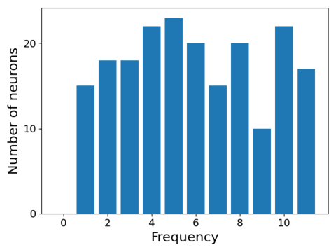
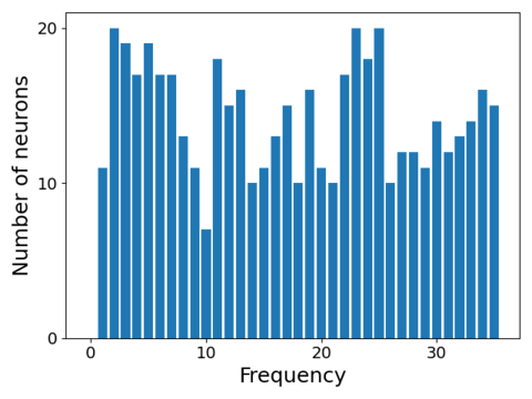
Moreover, we prove that every frequency is used by some neuron.

Thus, we have a resolution to the mystery in our setting:

Neural networks have a tendency to approach maximum margin solutions, and every maximum margin solution uses Fourier features.

Other Algebraic Tasks

Futhermore, we were able to extend our max margin analysis from modular addition (the cyclic group) to other finite groups, explaining the empirical results of Chughtai et al.! What is the ‘analogous’ result here? Basically, instead of all frequencies being used, all group representations are used. Furthermore, all neurons only use a single representation. For more details, see Section 6 of our paper.

We also derived results of a similar flavour for the sparse parity setting studied in works such as Daniely et al., Barak et al., and Edelman et al.

Beyond Algebraic Tasks?

We have shown that at least for simple algebraic tasks and simple neural networks, we can actually explain where features come from as a consequence of a known inductive bias of deep learning.

What are the prospects for understanding where features come from in general? If we can explain why neural networks prefer certain circuits over others, this can have significant implications:

• To what extent are learned circuits universal, and to what extent are they sensitive to the architecture and learning algorithm?
• Can we modify any aspects of the learning process to favor circuits that are more interpretable, robust, fair, or have other desired properties?
• In some cases, like training transformers on standard arithmetic, the “right” algorithm (i.e., one that generalizes off the training distribution) isn’t learned by default. If we can explain success stories of algorithm learning, can we also explain the failure cases?

We are hopeful that better understanding the inductive biases of neural networks will lead to a better understanding of feature learning.

1. Note that the Clock visualization algorithm still can be expressed using quadratic activations. One could further ask if changing to this architecture makes studying the solutions uninteresting, in the sense that this is the only solution it can express. In the Appendix of our paper, we show that the network can still express a memorizing solution even with quadratic activations.[↩]
2. L_2,3 norm : Consider a neural network of width $m$, and let the parameters associated with the $i^{th}$ neuron be represented by $u_i, v_i$ and $w_i$. Then $L_{2,3}$ norm of the network is defined as $\sum_{i=1}^m (||u_i||^2 + ||v_i||^2 + ||w_i||^2)^{3/2}$.
   In a technical sense, this norm is the “natural” norm for quadratic activations, in the same sense that $L_2$ norm is natural for ReLUs.[↩]
3. Let $\gamma^*$ represent the maximum normalized margin of the network with respect to a $|| \cdot ||$. Under mild assumptions on $f$, the normalized margin of the global minimizer of the loss given by $\mathbb{E}_{(x,y) \sim D} \ell(f(\theta; x), y) + \lambda \|\theta\|^r$ approaches $\gamma^*$ as $\lambda \to 0$. Here $\ell$ represents the standard cross-entropy loss and $r > 0$. [↩]